The Seasons They Are A-Changin’

A Century of Definitions and a Way Forward

Carter Bryson · Gary Cornwall

U.S. Bureau of Economic Analysis
The views expressed in this presentation are those of the authors and do not necessarily reflect the views of the Bureau of Economic Analysis or the U.S. Department of Commerce.

2026-08-01

Residual Seasonality: A Recurring, Cross-Agency Concern

Residual Seasonality in Core Consumer Price Inflation Federal Reserve Board • 2014

“The Phrase of the Day is ‘Residual Seasonality’ ” Wall Street Journal • 2015

U.S. says probe found problem in seasonal adjustment of GDP data Reuters • 2016

Residual Seasonality in GDP Growth Remains after Latest BEA Improvements Cleveland Fed • 2019

Assessing residual seasonality in published outputs UK Office for National Statistics • 2025

Residual Seasonality in Some Components of PCE Inflation Cleveland Fed • 2026

Residual seasonality recurs across agencies because the object is not agreed upon, not because any one producer is failing.

“Some of us looking for answers regarding seasonal analysis may feel as if we’re in a dark room looking for a black cat. That’s bad, but it’s not as bad as it could be. Pity the philosophers who are in a dark room looking for a black cat that isn’t there.” — Zellner et al. (1978, p. 451)

Twelve years of headlines, four different institutions, and the same complaint keeps resurfacing: residual seasonality. The Fed found it in core CPI, the Journal made it the phrase of the day, Commerce investigated GDP, the Cleveland Fed keeps finding it, and the UK’s ONS is now auditing for it. The recurrence is the tell — [click] this keeps happening across agencies because the object itself is not agreed upon, not because any one producer is doing a bad job. Zellner’s black cat captures the situation: we may all be in a dark room looking for a black cat — and it is worth asking whether the cat, a shared definition, is even in the room.

No agreed-upon definition

Tradition	Core object	Representative work
Regularity & repetition calendar-anchored	Seasonal means across a calendar partition	Falkner 1924; Kallek 1978; ESS Guidelines
Seasonal unit roots & stability ARIMA polynomial	Roots of the AR polynomial at seasonal frequencies	Hylleberg et al. 1990; Canova–Hansen 1995
Signal extraction unobserved components	Latent component St under an identifying restriction	Hillmer–Tiao 1982; Bell & Hillmer 1984; X-13ARIMA-SEATS
Spectral frequency-domain	Functional of the spectral density at seasonal frequencies	Nerlove 1964; Granger 1978

→ Each tradition is internally consistent — but none nests the others.

→ So analysts consult all of them, implicitly building the superset — a definition nobody wrote down.

Four traditions, a century apart, each with its own object. The point is not that any one is wrong — it is that they answer different questions, and practice quietly unions them. That superset is what we set out to formalize.

What do we mean by “seasonality”?

Before we can say what the tests disagree about, fix the taxonomy. The universe of time series splits into non-seasonal and seasonal. [click] Within seasonal, deterministic and stochastic seasonality are disjoint siblings — fixed calendar effects versus evolving ones. And seasonal unit roots are not a third species: they sit properly nested inside the stochastic box, as its extreme-persistence boundary case. This containment structure is exactly what the next slide’s test map is drawn over.

What are we testing for?

Every test in this literature commits to one null and one alternative among the four population objects on the right — and no two commit the same way. The presence bracket asks whether any seasonality exists; the type bracket presumes some and asks which kind. Two features of this map are corrections worth flagging: Soukup–Findley’s visual-significance statistic and McElroy’s 2021 ROOT statistic are mirror images inside the stochastic box — VS takes mild persistence as the null and strong as the alternative, ROOT exactly the reverse — and Franses (1994) is deliberately absent, because its null of periodic integration lies outside these four endpoints entirely. [click] Bryson–Cornwall joins the presence bracket: it shares the zero-seasonality null with those tests, but its alternative is the entire seasonal footprint — deterministic, stochastic, and seasonal unit roots at once — which is exactly the superset practitioners assemble informally.

Ambiguity Becomes Communication Opacity

Raw series transparent input

→

Judgment across frameworks implicit

→

X-13 Specification production default

→

Adjusted series opaque

“The QS diagnostic has limitation for pretesting (Findley et al. 2017). The main problem is that it may detect minor amounts of seasonal autocorrelation in a series, especially with a long series, and minor, though nonzero, amounts of seasonal autocorrelation do not reflect what we ordinarily think of as seasonality.” — Bell et al. (2022)

Who bears the cost?

• Within agencies. At BEA, BLS, Census, evidence is weighed across multiple frameworks (spectral diagnostics, HEGY, QS, visual significance) but the adjustment is applied by X-13 — which answers a different population question than most of the diagnostics that informed the decision to apply it.
• Between agencies. Different judgment conventions produce the same nominal output (“seasonally adjusted via X-13”) under different effective definitions. Comparable labels; incomparable objects.
• To data users. X-13 itself is transparent — code and manual are public — but the agency-specific spec that drives a given published series often is not. Users can read the engine; they cannot always read the configuration.

→ The superset exists but no one can point to it.

Having just seen the test map, here is what it does to production: a transparent raw series goes in, and before X-13 ever runs, an implicit judgment across those frameworks decides whether and how to adjust — that box is the dark one. The Bell quote hangs off the judgment box because it is the judgment step in the diagnostics community’s own words: QS, the workhorse diagnostic, flags statistically nonzero seasonal autocorrelation that “does not reflect what we ordinarily think of as seasonality” — so the analyst must overrule the formal statistic by appeal to an intuitive object no one has written down. Everyone pays: within agencies, the diagnostics that motivate adjustment answer a different population question than the tool that applies it; across agencies, identical labels hide different effective definitions; and users can read X-13’s engine but not always the configuration driving a given series. The superset exists but no one can point to it. [TODO: add the full Bell et al. (2022) reference to references.bib — not currently in the project bibliography.]

A Way Forward

What we build. A closed-loop framework that makes explicit what is currently assembled informally through analyst-level judgment:

• Definition. Seasonality as relative peak dominance.
• Test. Closed-form Logistic null via extreme value theory: no simulation, no bandwidth, no kernel.
• Adjustment. Stochastic Spectral Imputation (SSI) operates on the exact object the test measures.
• Design. Test and adjustment are logical conjugates, not bolted together.

What we find.

• After BIC pre-whitening, size is nominal across colored-noise nulls; power competitive with the best alternatives.
• SSI tracks X-13 in levels, preserves variance (VR \approx 1 vs. X-13’s \approx 0.75), and avoids spectral dips at seasonal frequencies.
• Housing starts and nonfarm payrolls: adjusted series pass independent diagnostics (ACF inside bands, no spectral dip, VR near 1).

→ We start by placing both the data and the definition in the frequency domain.

Here is the whole argument on one slide. We build four things: a definition, a test, an adjustment, and the design principle that makes the test and the adjustment logical conjugates rather than bolted-together procedures. The headline findings are nominal size after pre-whitening, competitive power, and an adjustment that preserves variance where X-13 loses roughly a quarter of it. Everything that follows unpacks this slide, starting by moving both the data and the definition into the frequency domain.

Two representations of the same series

Any finite-length series \{x_t\}_{t=1}^T admits two equivalent representations connected by the discrete Fourier transform:

d_x(\omega_j) = \sum_{t=1}^T x_t\, e^{-i\omega_j t}, \qquad x_t = \frac{1}{T}\sum_{j=0}^{T-1} d_x(\omega_j)\, e^{i\omega_j t}

at Fourier frequencies \omega_j = 2\pi j/T.

• Time domain orders observations by calendar position.
• Frequency domain decomposes variance by rate of repetition.
• Lossless. No information is gained or lost by changing coordinates.

Think of the time series as a relatively homogeneous object and the DFT as the centrifuge which separates it into its component parts.

The DFT is a lossless change of coordinates: same series, two languages. The time domain orders observations by calendar position; the frequency domain reallocates the same variance by rate of repetition. The centrifuge image is the one to leave them with — the series goes in whole, and the DFT separates it into component parts without gaining or losing any information.

The same seasonality in both domains

Time domain: monthly air passenger traffic

Frequency domain: periodogram

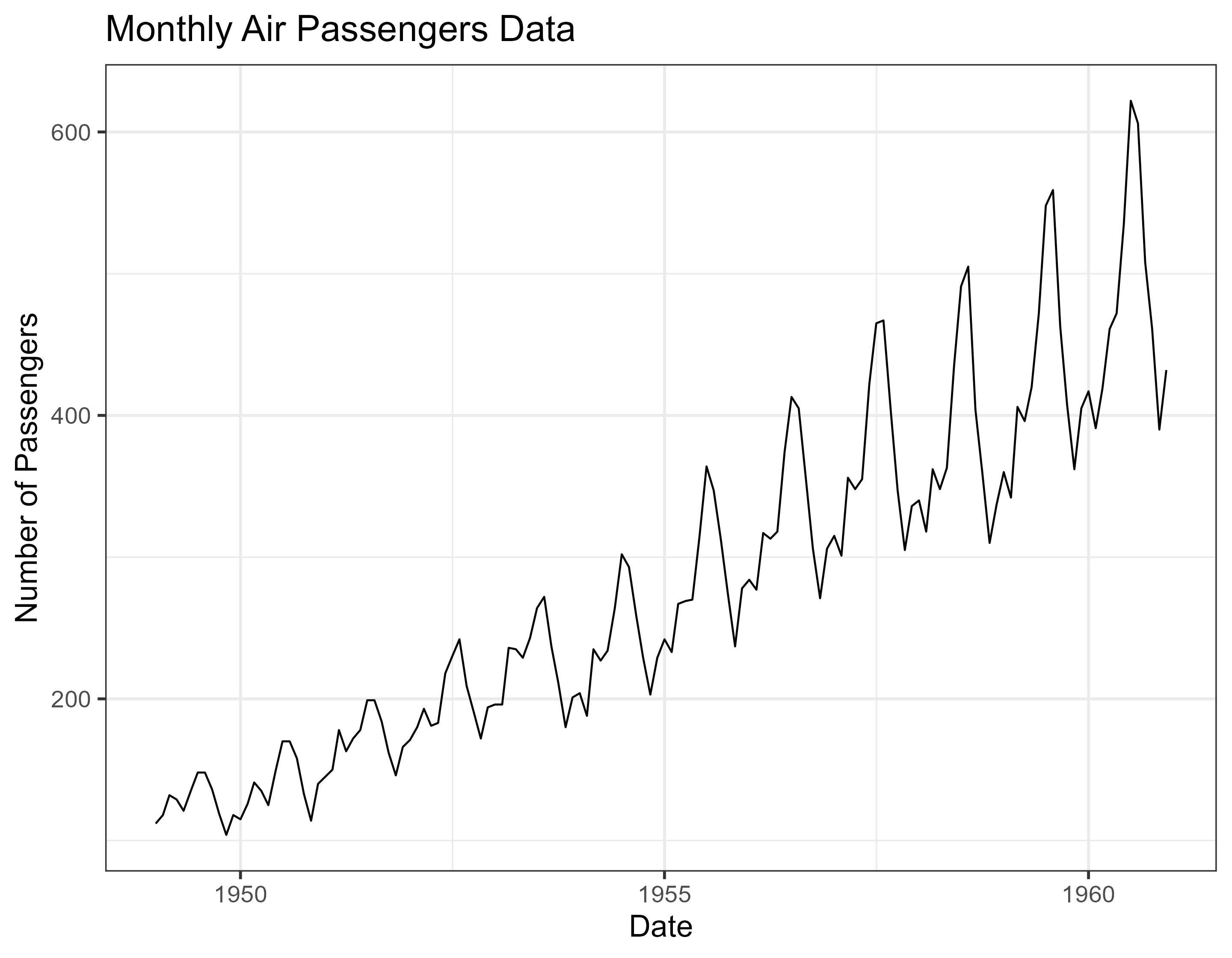
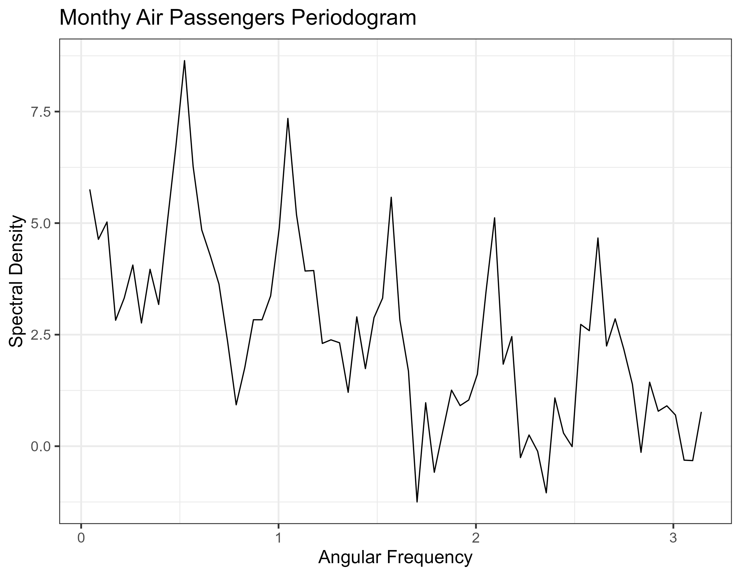
→ The annual cycle shows up both ways: as roughly twelve peaks per twelve years in the time plot, and as a sharp spike at the annual frequency (plus harmonics) in the periodogram.

→ Same structure, different coordinate language. In the frequency domain, periodicity becomes a property of specific frequencies rather than of calendar months — which is why we build the definition there.

Air passengers makes the equivalence concrete. Twelve years of monthly data show the annual cycle as repeated peaks in the time plot, and as a sharp spike at the annual frequency plus its harmonics in the periodogram. Same structure, different coordinate language. In the frequency domain periodicity is a property of specific frequencies rather than of calendar months, which is exactly why we build the definition there.

Why define seasonality in the frequency domain?

• Calendar-invariant. Repetition rate is universal. Gregorian, fiscal, and lunar calendars collapse to the same frequency representation.
• Model-free superset. Deterministic, stochastic, and unit-root seasonality all manifest as excess spectral mass at seasonal frequencies. Time-domain frameworks typically commit to a specific generating structure; the frequency-domain definition does not.
• Natural variance decomposition. Seasonality becomes a statement about how variance is allocated across frequencies — not about mean structure or autocovariance at specific lags.
• Moving holidays. Effects whose expected repetition rate sits near a seasonal rate (e.g., Easter, Ramadan) concentrate spectral energy near seasonal frequencies and are captured. Effects whose rate sits elsewhere (trading day, pay-period artifacts) are handled separately as pre-regressors before the DFT.
• Robust to outliers. An additive outlier spreads energy approximately broadband rather than concentrating at any particular frequency. Relative comparisons between seasonal and non-seasonal frequencies are largely preserved. Time-domain partition tests are distorted directly by outliers in specific periods.

One caveat. The periodogram is an inconsistent estimator of the spectral density. We don’t try to fix this; we exploit it.

Five reasons to define seasonality here: it is calendar-invariant; it is a model-free superset covering deterministic, stochastic, and unit-root seasonality; variance decomposition is the natural object; moving holidays whose rates sit near seasonal frequencies are captured while trading-day effects are pre-regressed out; and additive outliers spread roughly broadband, so relative comparisons survive. The caveat sets up the entire test: the periodogram is inconsistent, and instead of fixing that we exploit it.

A definition you can test

Non-technical. Among all of a series’ possible repeating cycles, the ones associated with chosen cycles of interest are demonstrably larger than the others.

Technical. Relative to a set of chosen cycle lengths, the highest peak in the spectral density occurs near one of those cycles rather than at any other.

We derive a test statistic with a clean asymptotic null — the distance between the periodogram’s max height in seasonal vs. non-seasonal bins.

\begin{aligned} \textcolor{#9EA2A2}{\widehat{\Delta}}(z;\textcolor{#004C97}{\mathcal{P}},N,M) \;:=\;& \max_{m \in \textcolor{#007D8A}{\mathcal{M}_1}(\textcolor{#004C97}{\mathcal{P}},N;M)} b_m(\textcolor{#D86018}{I_T}) \\[2pt] \;-\;& \max_{m \in \mathcal{M}_0(\textcolor{#004C97}{\mathcal{P}},N;M)} b_m(\textcolor{#D86018}{I_T}) \end{aligned}

Under H_0:

\textcolor{#9EA2A2}{\widehat{\Delta}} \overset{d}{\rightarrow} \mathrm{Logistic}\bigl(\tau \log(N_1/N_0),\,\tau\bigr)

via EVT on periodogram ordinates.

Read the non-technical definition first — the color coding carries through to the technical version and into the statistic itself: orange is the spectral object, blue the chosen cycles, teal the association, gray the comparison. The statistic is simply the distance between the tallest seasonal-bin ordinate and the tallest non-seasonal ordinate. Under the null that distance converges to a Logistic with known location and scale — no simulation, no bandwidth, no kernel.

The population object: the partition

Fix an ex ante set of fundamental periods \mathcal{P} \subseteq \{1,\dots,P_{\max}\}. Non-annual fundamentals (e.g. quadrennial cycles) are handled identically; for now assume \mathcal{P}=\{1\}.

Harmonics. For p \in \mathcal{P} and N observations per year,

\Omega_p(N) = \Bigl\{\tfrac{2\pi k}{pN} : k = 1,\dots,\lfloor pN/2 \rfloor\Bigr\}, \qquad \Omega_G(\mathcal{P},N) = \bigcup_{p \in \mathcal{P}} \Omega_p(N).

Monthly (N=12,\ \mathcal{P}=\{1\}): \Omega_G = \{\pi/6,\ \pi/3,\ \pi/2,\ 2\pi/3,\ 5\pi/6,\ \pi\}.

Partition. Divide (0,\pi] into M equal-width bins B_m and label:

\mathcal{M}_1 = \{m : \mathrm{int}(B_m) \cap \Omega_G \ne \emptyset\}, \qquad \mathcal{M}_0 = \{1,\dots,M\} \setminus \mathcal{M}_1.

makePartition({mode: "bins"})

The partition is the design object, and it is fixed ex ante — before any series is seen. Fix the fundamental periods, collect their harmonics — six of them monthly, the Nyquist pi included as implemented in freqseas — cut the interval from zero to pi into M equal-width bins, and label a bin seasonal exactly when it contains a harmonic. Drag M across the boundary-safe values 11, 19, 23, 31: the bins recolor, the count of non-seasonal bins goes 5, 13, 17, 25, but the harmonic ticks never move and there are always exactly six seasonal bins, one per harmonic. Note what is deliberately absent: there is no data on this slide. Nothing here has been estimated, nothing has been observed. This is purely the design object, which is why the M slider is the only input. The next two slides add the two things that are missing, in order — first a spectral density to measure over these bins, then a single sample drawn from it — and the slider carries across all three, so whatever M you pick here is the M you see there. The design resolution is a choice, not a tuning knob: the M-sensitivity table in the appendix backs that with empirical size.

The population object: Δ

Comparing the elevations of two mountain ranges, relative to a common sea level.

Bin maximum. b_m(f_Z) \;:=\; \sup_{\omega \in B_m} f_Z(\omega).

Population separation:

\Delta(f_Z;\mathcal{P},N,M) \;=\; \underbrace{\max_{m\in\mathcal{M}_1} b_m(f_Z)}_{\text{largest seasonal-bin peak}} \;-\; \underbrace{\max_{m\in\mathcal{M}_0} b_m(f_Z)}_{\text{largest non-seasonal peak}}.

makePartition({mode: "sdf"})

Definition. \{Z_t\} is seasonal relative to (\mathcal{P},N,M) iff \Delta(f_Z;\mathcal{P},N,M) > 0.

Relative, not absolute: captures narrow peaks and diffuse seasonal energy that remains concentrated within the seasonal bins. \Delta is indexed by the design resolution M.

The population object compares the elevations of two mountain ranges relative to a common sea level. Take the highest peak of the spectral density over the seasonal bins, the highest over the non-seasonal bins, and call the gap Delta. The series is seasonal relative to the design exactly when Delta is positive. It is a relative statement, so it captures narrow peaks and diffuse but concentrated seasonal energy alike, and it is indexed by the design resolution M. The density here is synthetic, not estimated — still no data, this is the population object. The M slider is live and shared with the slides either side, so the bins you chose a moment ago are the bins being measured now. Note the vertical axis is linear, so the black arrow’s length simply is Delta. One thing worth saying out loud if anyone drags the slider: Delta does not move. That is correct, and it is the point of the design. The seasonal supremum is the pi/2 spike and the non-seasonal supremum is the tall broad bump, and because that bump sits midway between two harmonics it stays strictly inside a non-seasonal bin at every resolution in this set. So Delta is invariant here by construction; the M-dependence lives in the sample statistic and in the critical value, which is exactly where the next two slides put it.

The sample analog

For a finite sample \{z_t\}_{t=1}^T, we estimate f_Z with the periodogram:

I_T(\omega_j) \;=\; \frac{1}{T}\left|\sum_{t=1}^T \tilde{z}_t\, e^{-i\omega_j t}\right|^2, \qquad \omega_j = \tfrac{2\pi j}{T},\ \ j = 1,\dots,\lfloor (T-1)/2 \rfloor.

Within-bin maximum. Let \mathcal{J}_m = \{j : \omega_j \in B_m\}. Then b_m(I_T) := \max_{j \in \mathcal{J}_m} I_T(\omega_j).

Sample statistic:

\widehat{\Delta}(z;\mathcal{P},N,M) \;=\; \underbrace{\max_{m \in \mathcal{M}_1} b_m(I_T)}_{\text{largest seasonal-bin ordinate}} \;-\; \underbrace{\max_{m \in \mathcal{M}_0} b_m(I_T)}_{\text{largest non-seasonal ordinate}}.

makePartition({mode: "sample"})

Next: under H_0 the ordinates are \approx i.i.d. exponential; we don’t correct this, we exploit it.

The sample version swaps the spectral density for the periodogram, and sup for max over the ordinates falling in each bin. Everything else is identical: same bins, same two maxima, same gap. What is on screen is one draw from exactly the density on the previous slide — each ordinate is f at that frequency times an independent Exp(1), seeded once, so the slider repartitions this one sample and never redraws it. Two things to point at. First, the axis rescales: the faint orange curve is the same density as the slide before, but the ordinates run several times above it, because a periodogram ordinate is exponential around f, not equal to f — that noise is the whole reason this is a testing problem and not an arithmetic one. Second, Delta-hat is 0.51 at M = 11, 23 and 31, and 0.74 at M = 19, against a population Delta of 0.73 at every one of them — the gap is sampling error, nothing else. Both are in the readout, so you can say the number. Do not oversell the M = 19 agreement: the default happens to be the one resolution where Delta-hat lands almost exactly on Delta, and sliding off it shows the honest 30 percent undershoot. That gap is what needs a distribution, and the next slide supplies it — deliberately no critical value and no verdict here yet. The closing line is the hinge: under the null the ordinates are approximately i.i.d. exponential, and rather than correcting that inconsistency we exploit it.

The null distribution

Under H_0: Z_t \sim \mathrm{WN}(0,\sigma^2). Then at Fourier frequencies,

\frac{I_T(\omega_j)}{\tau} \;\Rightarrow\; \mathrm{Exp}(1), \qquad \tau = \sigma^2,

independently across distinct \omega_j (Politis & McElroy, 2019).

With N_g = |\mathcal{J}_g|, classical EVT gives the chain

\mathrm{Exp}(1)^{\otimes N_g} \;\xrightarrow{\ \max\ }\; \mathrm{Gumbel}(\tau\log N_g,\, \tau) \;\xrightarrow{\ \text{diff.}\ }\; \mathrm{Logistic}\bigl(\tau\log(N_1/N_0),\, \tau\bigr),

with independence across disjoint \mathcal{J}_1, \mathcal{J}_0, so

\boxed{\ \widehat{\Delta}(z;\mathcal{P},N,M) \,\big|\, H_0 \;\Rightarrow\; \mathrm{Logistic}\!\left(\tau\log\tfrac{N_1}{N_0},\,\tau\right)\ }

makeNullDist({})

full derivation →

Under white noise the periodogram ordinates are asymptotically independent exponentials, so classical extreme value theory does all the work. The maximum of exponentials is Gumbel; the difference of two independent Gumbels with a common scale is Logistic. The widget runs the whole chain live and honestly labeled: each draw scatters 516 fresh Exp(1) ordinates on the real payrolls grid — seasonal bins shaded, N1 = 165 orange, N0 = 351 gray — the two maxima flash with their gap, and Delta-hat drops into the histogram over the exact Logistic null with location log of N1 over N0 and scale one. At slow speed narrate one draw end to end; then push the speed slider and let a few thousand draws pile up — the histogram locks onto the blue curve, and the running rejection counter sits at five percent against the shaded tail. The point: no simulation is needed in practice — the closed form is the entire critical-value apparatus — but when you do simulate, the closed form is exactly where the draws land. The statistic is the plain difference of standardized ordinates, tau-hat equals one; everything on screen is seeded and deterministic.

Practical workflow

1. Pre-whitenfit nonseasonal ARIMA by BIC; take residuals \hat{e}_t

Why pre-whiten? Colored-noise power sits in non-seasonal bins (low-frequency under AR(1)+, high-frequency under AR(1)-), inflating \max_{\mathcal{M}_0} b_m and shrinking \widehat{\Delta}. Raw \widehat{\Delta} rejects 0.3% of the time on AR(1), \phi=0.8; BIC pre-whitening restores size to 0.043–0.051. size table → In the software implementation this step has matured into M0-Whittle whitening — a de-biased Whittle AR fit that excludes seasonal-neighborhood ordinates (“Stage 0”) — same role, sharper tool.

↓

2. Standardize(\hat{e}_t - \bar{e})/s_e enforces \tau = 1

Why standardize? With \tau=1 the null collapses to \mathrm{Logistic}\bigl(\log(N_1/N_0),\, 1\bigr): a single known distribution whose only data-dependent input is the partition.

↓

3. Apply testcompute \widehat{\Delta}; reject if > c_{1-\alpha}

How sensitive to M? Empirical size holds in [0.046, 0.054] across M \in \{11, 19, 23, 31\} under white noise. M-sensitivity →

Three steps in practice. Pre-whiten, because colored noise piles power into non-seasonal bins and destroys size — the raw statistic rejects 0.3 percent of the time on a strong AR(1), while BIC pre-whitening restores size to nominal; in freqseas this step has matured into M0-Whittle whitening, Stage 0 of the pipeline. Standardize, so that tau equals one and the null collapses to a single known Logistic whose only data-dependent input is the partition. And the choice of M barely matters: empirical size stays within half a point of nominal across M from 11 to 31.

Simulation evidence: well-sized with competitive power

Size. Empirical null matches \mathrm{Logistic}(\tau\log(N_1/N_0),\tau) almost exactly.

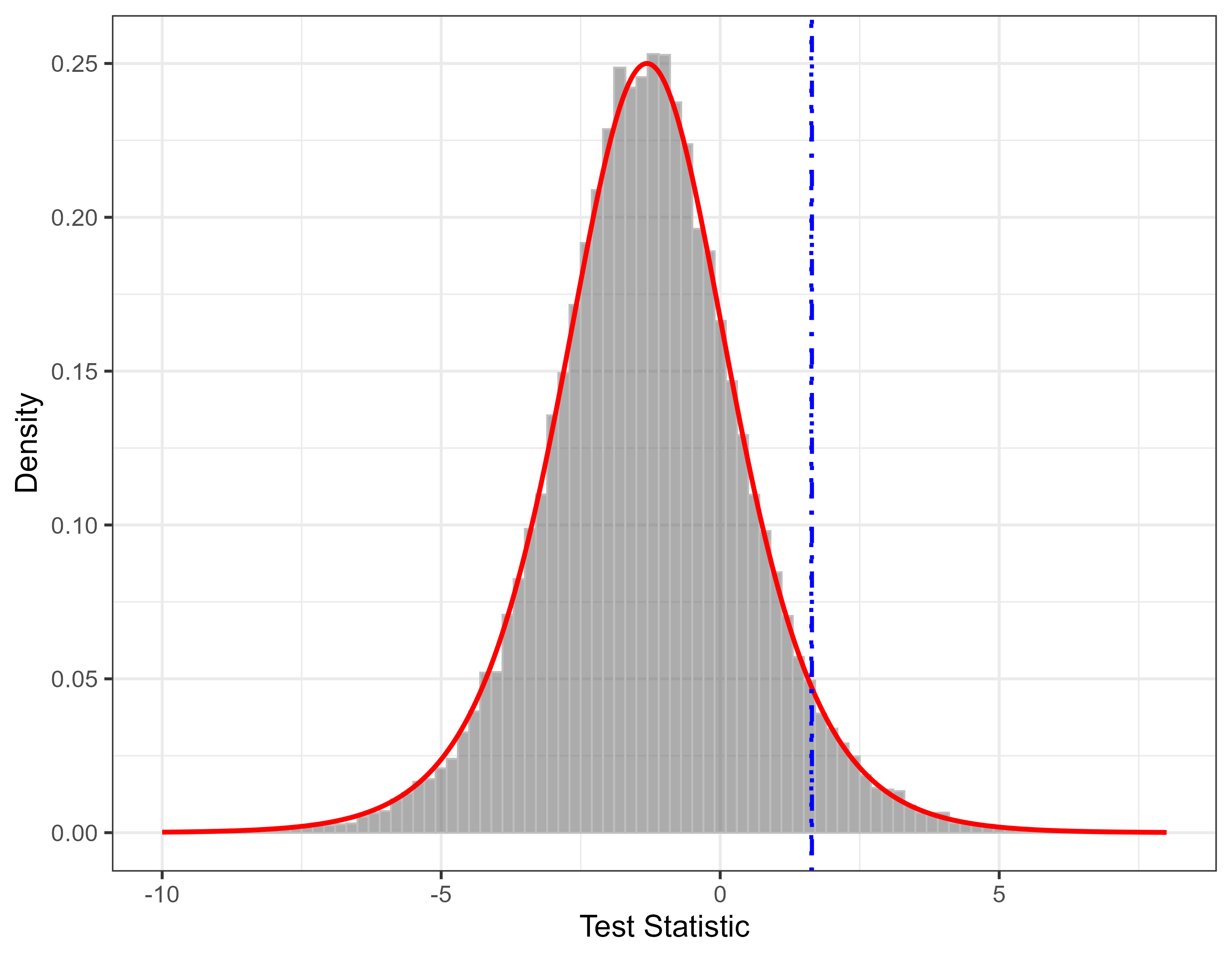
Monthly, T=200, 50,000 replications. Vertical line: nominal 5% value.

Power. Competitive overall; dominates in quarterly and in the stationary-stochastic regime where BHs and CH fail.

	\widehat{\Delta}	BHs	CH	QS	VS
Monthly, stoch. seas. (ρ = 1), σ²η = 0
σκ = 0.02	0.72	0.40	0.26	0.88	0.75
σκ = 0.03	0.95	0.75	0.53	0.99	0.96
Monthly, stoch. stat. (ρ = 0.95), σ²η = 0.5
σκ = 0.03	0.65	0.06	0.05	0.83	0.43
Quarterly, stoch. seas., σ²η = 0.5
σκ = 0.03	0.61	0.38	0.36	0.54	0.54

T=200; N=12/4, M=23/7, P=1. Full tables in appendix.

No bandwidth, no kernel, no simulated critical values — just the Logistic distribution.

Two panels. On the left, the empirical null at T equal to 200 sits on the theoretical Logistic almost exactly — the asymptotics arrive early. On the right, power is competitive overall, and the test dominates exactly where the classic alternatives fail: the stationary-stochastic regime kills BHs and CH, and in quarterly designs we lead the field. The applause line is the closer — no bandwidth, no kernel, no simulated critical values, just the Logistic distribution.

From test to adjustment: the logical conjugate

What the test measures. Excess seasonal-bin spectral power: \widehat{\Delta}(z;\mathcal{P},N,M) > 0.

The gap most procedures leave open. Adjustment filters (X-13, SEATS, STL) target different population objects than any specific seasonality test. The filter does its job; the test does its job — but the two don’t speak the same language.

What our adjustment should do. Remove exactly the excess the test detects: leave the adjusted series x^*_t with

\widehat{\Delta}(x^*;\mathcal{P},N,M) \;\approx\; 0

by construction, while preserving the non-seasonal spectral floor.

The logical conjugate. Test and adjustment share a partition and target the same object. \widehat{\Delta}(x^*) \approx 0 holds by construction; independent diagnostics (ACF inside bands, no spectral dip, variance ratio near 1) provide the empirical check.

Operationalization: Stochastic Spectral Imputation (SSI).

This is the hinge of the talk: most shops run a test from one tradition and a filter from another, so the filter removes an object the test never measured. Our design requirement is that the adjustment remove exactly the excess the test detects — re-run the test on the adjusted series and it returns approximately zero by construction. That makes test and adjustment logical conjugates over the same partition, and the independent diagnostics keep the claim honest rather than circular. SSI is the operator that delivers it.

Stochastic Spectral Imputation

Every seasonal-bin ordinate is reset to a drawn donor level from the non-seasonal floor — the paper’s SSI, as implemented in freqseas, on BLS nonfarm payrolls.

makeSurgery({})

explore →

The widget replays a genuine freqseas run on payrolls — nothing is computed in the browser; every draw was made by the package in R. The algorithm in three moves (details at app-ssi-algo): Setup — DFT the whitened series; seasonal-bin ordinates are targets, quiet ordinates below the quantile threshold are donors. Imputation — each target’s magnitude is reset to a drawn donor’s level; on this classic path each target keeps its own phase (the paper’s zero-phase story — the minimum-gain phase machinery belongs to the package’s band branch, shown as the deterministic comparison in the explore appendix). Finalize — conjugate symmetry, inverse DFT, recolor, restore levels. Press Adjust: the setup flash rings the 165 targets and lights the donor pool under the dashed threshold; the first ordinate of each of the first three harmonics plays slowly — donor flashes, ordinate drops to the donor level, and the extracted sinusoid ripples across the time panel; then the remaining ordinates cascade through in a couple of seconds, harmonic labels flashing as each bin empties. Displayed levels are benchmarked throughout: yearly totals are forced to the NSA sums pro-rata via freqseas::benchmark_totals — the accounting constraint imposed by X-13 practice and the national accounts. At the close the reconstruction snaps to the exact package output, the X-13 overlay draws in, and the \widehat{\Delta} chip flips: 116.4, p below machine precision, reject — to p = 0.97 on the benchmarked series, fail to reject. The same test that found the seasonality certifies its removal. Stochasticity: a fresh donor draw each run — fix the seed for production, or average replications for uncertainty bands; the reseed control in the appendix explore instance shows exactly that. If the widget is down, fall back to the static twin in the source.

Evaluating SSI against X-13

Adjustment quality is multidimensional. X-13 is known to over-smooth and create spectral dips at seasonal frequencies. We weight four criteria by what they actually reveal:

• Variance ratio \mathrm{Var}(\hat e)/\mathrm{Var}(\epsilon). Should \approx 1. X-13 typically \approx 0.75: systematic under-variance.
• Spectral dip. Mean |\hat f_{\hat e}(\omega) - \hat f_\epsilon(\omega)| within seasonal bins. SSI imputes to the noise floor; X-13 undershoots it.
• Correlation with \epsilon_t. Dynamic fidelity of innovations, not just magnitudes.
• Time-domain MAE (secondary). Over-smoothing reduces MAE mechanically when bias is comparable — interpret jointly with the variance ratio.

Representative case
BSM, monthly, \rho = 0.95, \sigma_\kappa = 0.03.

	SSI	X-13
Variance ratio	0.98	0.76
Spectral dip	0.21	0.38
Corr(ê, ε)	0.90	0.82
MAE	1.11	1.03

Bold: closer to target. → DGP

Full panels: A (UR) · B (SS) · C (Det)

The headline number is the variance ratio: X-13’s 0.76 is systematic under-variance — over-smoothing — while SSI sits at 0.98. The spectral dip tells the same story in the frequency domain: X-13 digs below the noise floor at seasonal frequencies, SSI imputes to it. MAE is grayed on purpose: over-smoothing lowers MAE mechanically, so on its own it rewards exactly the failure mode — read it jointly with the variance ratio. Full panels for the unit-root, stochastic-stationary, and deterministic DGPs are one link away in the appendix.

Combined workflow — and its operational form

1. Pre-data design: choose α and M

↓

2. Test workflow

→ pre-whiten→ standardize→ apply test

Stage 0 · whiten A · detect

↓

\widehat{\Delta} > c_{1-\alpha} ?

B · specify — line vs band identify — declared phase rule

no ↓

No adjustment
not seasonal at level α

yes ↓

3. SSI workflow
stationarize → apply SSI → restore levels

operate · surgery

On α: larger \alpha ⇒ smaller c_{1-\alpha} ⇒ more series classified as seasonal; standard choice 0.05 — pre-specify before observing data, or \alpha becomes a tuning knob.

On M: design resolution of the bin partition; defaults M = 2N-1 (monthly → 23, quarterly → 7); empirical size is insensitive to M across reasonable choices.

Status. The detect test and SSI are the paper. Stage B and the identification layer are active development: the line-vs-band specification test and the phase rule (not testable at second order — a declared identification) are experimental.

One slide, about two minutes. First beat is the paper’s workflow: fix alpha and M before seeing data, test, decide, and adjust only on rejection. Second beat: the same boxes wear their freqseas stage names — whiten, detect, specify, identify, operate — with specification and identification slotting in between test and adjustment. If asked why the SSI leg is simpler than the test leg: the asymmetry is intentional — the test must defend a null distribution (approximately i.i.d. exponential ordinates, hence whitening and standardization), while the adjustment should operate on whatever non-seasonal structure the observed series actually has, preserving the features the analyst wants to keep. Close on the status line: detect and SSI are the paper; specification and the phase rule are the active edge.

Nonfarm payrolls: SSI in production conditions

Full period 1990–present

COVID zoom 2018–2022

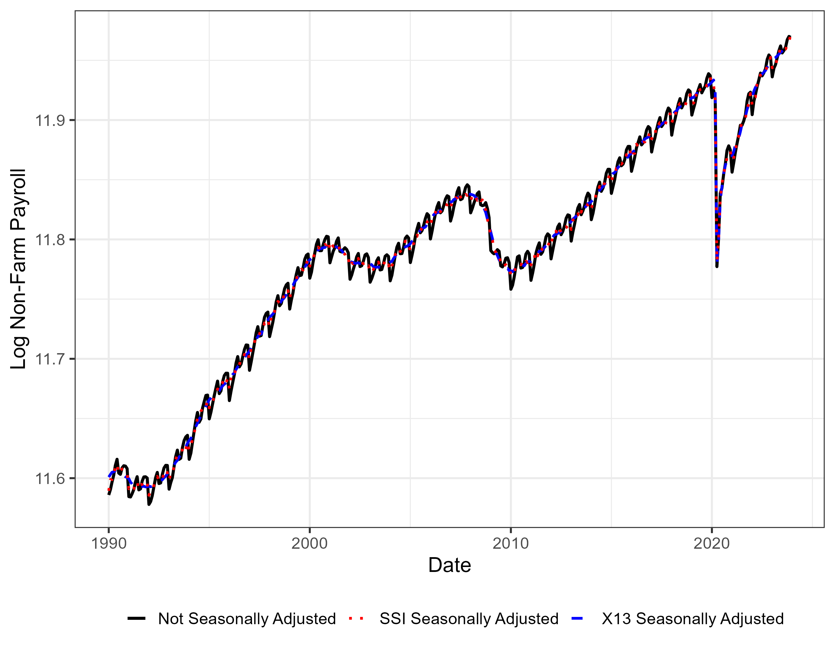
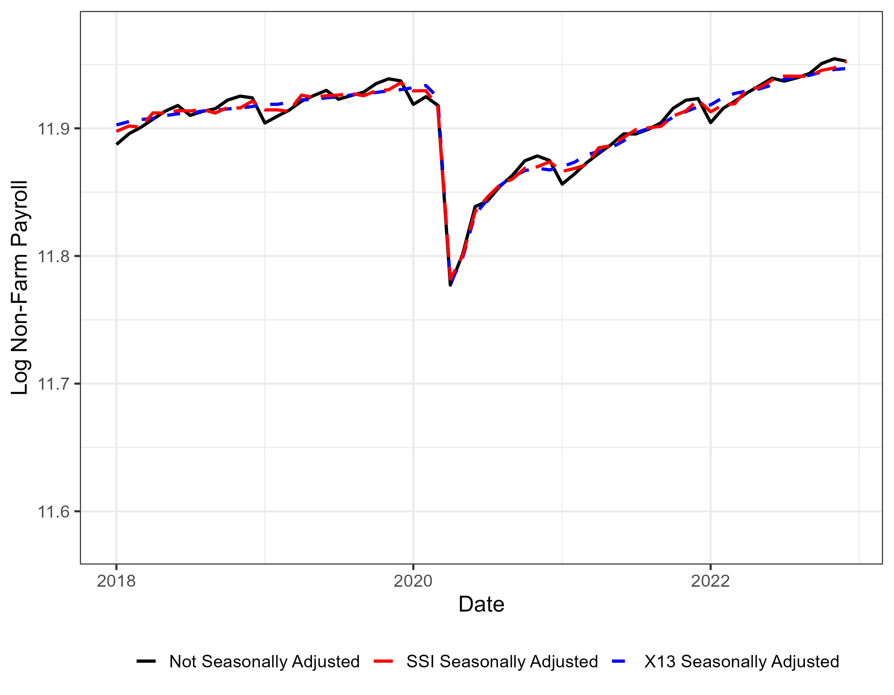
→ SSI and X-13 produce nearly identical level series — consumers of the adjusted data would not detect the change at scale.

→ The COVID shock — historically large month-over-month swings — handled mechanically, with no judgmental adjustments: reproducibility and auditability at production scale.

We start with CES nonfarm payrolls — your series — and the hardest stretch it has faced. Over the full 1990–present period, SSI and the published X-13 series are nearly identical in levels; a consumer of the adjusted data would not detect the change. The point to land is the second one: the COVID months produced historically large month-over-month swings, and SSI absorbed them mechanically, with no judgmental interventions — the property that matters for reproducibility and auditability in a production system. Expect follow-ups here on concurrent adjustment and revisions policy; the answer is that a mechanical operator makes the revision path itself auditable.

Payrolls — diagnostics

Autocorrelation (seasonal lags highlighted)

Periodogram (\log_{10}; seasonal bins highlighted)

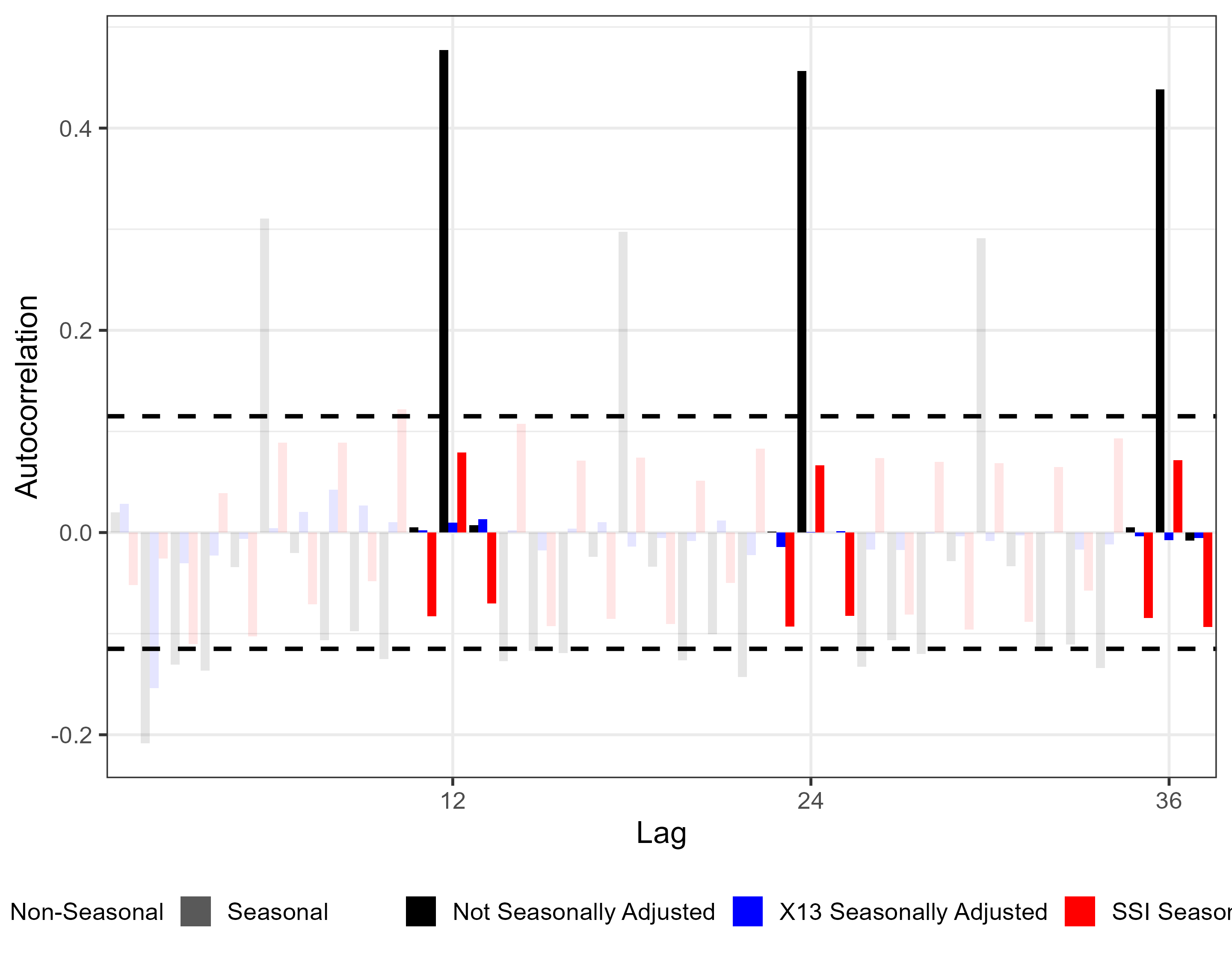
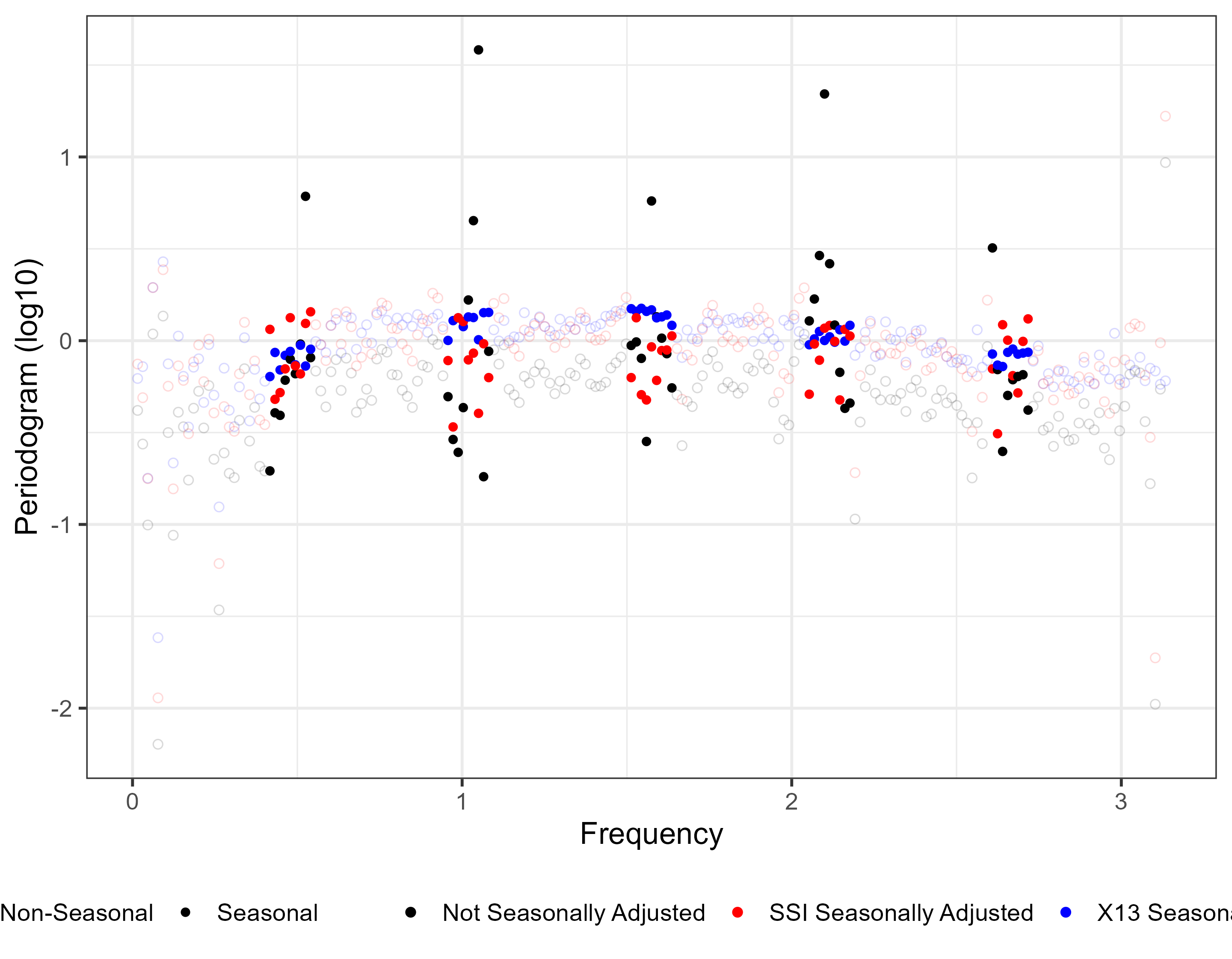
→ ACF: both SSI and X-13 bring seasonal autocorrelations to insignificance. SSI introduces a mild alternating pattern (trigonometric imprint); neither value is significant.

→ Periodogram: over-smoothing by X-13 is visible directly — dispersion in seasonal bins is much tighter than in non-seasonal bins. SSI matches the floor across the board.

Two diagnostics on the same adjustment. On the ACF, both methods do their job — seasonal autocorrelations fall inside the significance bands; SSI’s mild alternating pattern is the trigonometric imprint of the imputation and is itself insignificant. The periodogram is the more revealing panel: X-13’s over-smoothing shows up directly as unnaturally tight dispersion in the seasonal bins, while SSI’s ordinates match the non-seasonal floor across the board — replaced energy that looks like the rest of the spectrum.

Housing starts

Full period 1990–present

Autocorrelation (seasonal lags highlighted)

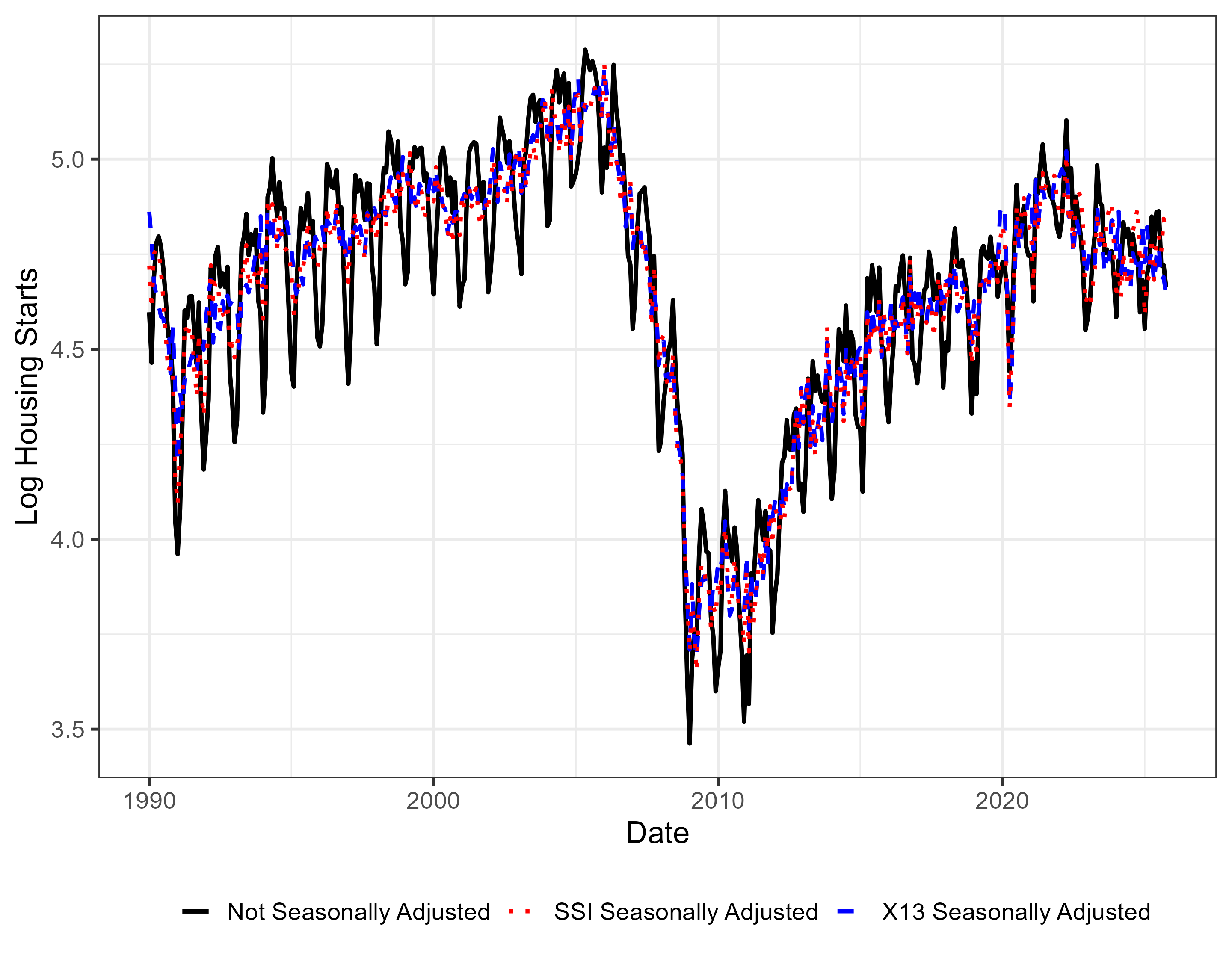
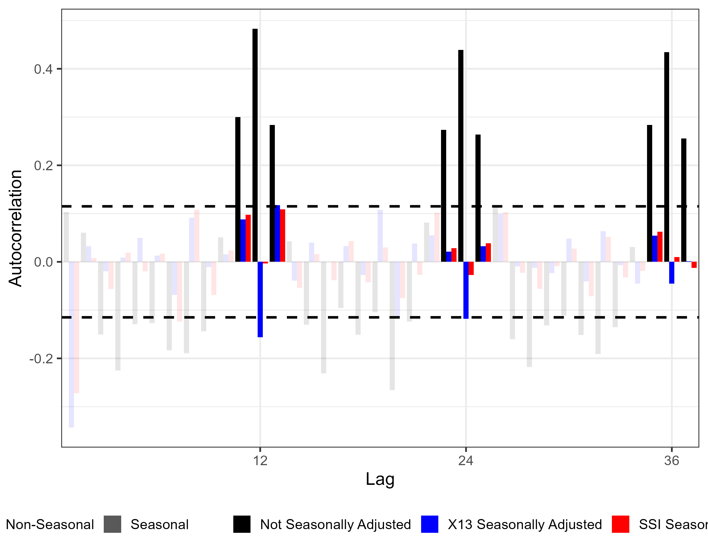
→ SSI tracks the published X-13 series closely and stays slightly more volatile — by design: less over-smoothing.

→ X-13 overcorrects at lag 12 — strongly positive in the raw series, strongly negative after X-13. SSI brings lags 12, 24, 36 inside the bands.

periodogram diagnostic →

Second series: Census housing starts, a strongly seasonal construction series. Same pattern in levels — SSI tracks the published X-13 series closely while staying slightly more volatile, which is a feature, not a bug: less over-smoothing. In 2020, X-13 overstates the Q1 level and the subsequent contraction; SSI is more moderate, preserving the pandemic signal rather than absorbing it into “seasonal.” On the ACF, X-13 actually overcorrects lag 12 — flipping it from strongly positive to strongly negative — while SSI brings the seasonal lags inside the bands. The periodogram diagnostic is in the appendix if it comes up.

Empirical takeaways

Level series tracks X-13

No disruption to published magnitudes; transition risk appears low.

Less over-smoothing

Volatility closer to the underlying irregular, variance ratio nearer 1.

Clean spectral diagnostics

No dip at seasonal frequencies; ACF inside bands without over-correction.

Mechanical at scale

No judgmental adjustments during the COVID shock: suitable for production workflows and scale.

Closed loop, empirically

Test rejects on both raw series; fails to reject on either SSI-adjusted series. ACF and periodogram diagnostics corroborate.

Five results from the two applications. Levels track X-13, so transition risk is low; volatility sits closer to the underlying irregular; the spectral diagnostics are clean, with no seasonal trough and no ACF over-correction; and the whole thing ran mechanically through COVID. The last bullet is the one to end on: the loop closes empirically — the test rejects on both raw series and fails to reject on either SSI-adjusted series, with the ACF and periodogram diagnostics corroborating. Definition, test, and adjustment answering the same question against the same object, on real production data.

freqseas: the framework as software

library(freqseas)
tst <- seas_test(AirPassengers)   # detect + specify
adj <- seas_adjust(AirPassengers) # ...→ identify → operate

freqseas seasonality test
 decision: seasonal (detection p = 2.86e-08, alpha = 0.05)
 spec: line (shoulder p = 0.219, phase R = 1.00)
 M = 19 (suggest_M, offset-free) | whitener: d = 0, AR(1) on M0 ordinates
SSI seasonal adjustment (line)
 phase rule: minimum  [declared identification]
 imputation: bootstrap, B = 1, targets = harmonics (6), seed = none
 post-adjustment detection p = 0.182

Actual package output (v0.0.0.9000), lightly abridged for the slide. The adjustment is stochastic by default — pass seed to pin the draw.

Solid — the paper

• the \widehat{\Delta} detect test (EVT chain, Logistic null)
• SSI surgery (operate)
• ts / tsibble methods; keyed series mapped independently

Experimental — in motion

• line-vs-band specification test
• declared phase identification (minimum vs zero)
• benchmarking to annual totals
• fixed-factor / revisions workflow

→ Package under active development — collaboration welcome.

Everything in the talk is one call each: seas_test runs whiten–detect–specify, seas_adjust runs the full pipeline through the surgery. The printed output on the left is a real run on AirPassengers — the EVT decision with its p-value, the line/band specification, the whitener record, then the phase rule tagged explicitly as a declared identification and the self-check: post-adjustment detection p of 0.18, the closed loop in software. Be candid about the two tiers: the detect test and SSI carry the paper’s theory; specification, phase identification, benchmarking, and the revisions workflow are experimental. BLS runs the largest seasonal-adjustment production system there is — the collaboration line is a genuine invitation, not a courtesy.

What to take away

A definition that can be tested. Seasonality as relative peak dominance in the frequency domain: a single population object, explicit about its primitives, stated in both plain and technical language.

A closed loop: definition → test → adjustment. \widehat{\Delta} with a Logistic null (no bandwidth, no kernel, no simulation) plus SSI, the adjustment operator aligned with the test’s population object. Coherence-by-construction — achievable, but not automatic.

Why it matters. Statistical offices publish millions of series under real resource constraints — BEA alone ≈ 4M across NIPA and the satellite accounts. Robustness, transparency, minimal parametric commitment, and scalability are design requirements, not luxuries — and a test and adjustment that answer the same question against the same object make the work easier to communicate: within agencies, between them, and with the public.

An invitation. A proof of concept that epistemic closure in seasonal adjustment is achievable. We invite researchers working in the time domain, state space, or elsewhere to build equivalent closed loops in their preferred formalism — so the field can communicate about definitions, not just procedures.

Land the three bullets slowly — they are the talk. If time allows, restate the recap framing: the problem is definitional and communicative, and practitioners already build the superset definition implicitly — we formalized it. The scale point makes the design constraints concrete: at millions of series, robustness, transparency, minimal parametric commitment, and scalability are requirements, not luxuries. End on the invitation: equivalent closed loops in other formalisms would let the field argue about definitions instead of procedures.

Thank you

The Seasons They Are A-Changin’: A Century of Definitions and a Way Forward

Working paper · U.S. Bureau of Economic Analysis

carter.bryson@bea.gov · gary.cornwall@bea.gov

The views expressed in this presentation are those of the authors and do not necessarily reflect the views of the Bureau of Economic Analysis or the U.S. Department of Commerce.

Thank the audience, point at the emails, and open the floor. Likely Q&A territory: concurrent adjustment and revisions policy, moving holidays and trading day, short samples, and how our diagnostics relate to the QS and M-statistics culture — the appendix bank and the freqseas notes cover each of these. If the software slide sparked interest, offer to follow up with the package and the working paper directly.

Appendix

Reached via links from the main deck — press Esc / O for the slide overview to return.

The null distribution — full derivation

1. Periodogram ordinates under H_0. For Z_t \sim \mathrm{WN}(0,\sigma^2), let \tau := \sigma^2. At Fourier frequencies \omega_j = 2\pi j/T, j \ge 1, I_T(\omega_j)/\tau \;\xrightarrow{d}\; \mathrm{Exp}(1), with asymptotic independence across distinct \omega_j (Politis & McElroy, 2019).

2. EVT for i.i.d. exponentials. For Y_1,\dots,Y_N \overset{\mathrm{iid}}{\sim} \mathrm{Exp}(1), \Pr\bigl(\textstyle\max_i Y_i - \log N \le x\bigr) \to e^{-e^{-x}}. Scaling by \tau: for M_g := \max_{j \in \mathcal{J}_g} I_T(\omega_j), \frac{M_g - \tau\log N_g}{\tau} \;\Rightarrow\; \mathrm{Gumbel}(0,1), so M_g \approx \mathrm{Gumbel}(\tau \log N_g,\, \tau).

3. Independence of M_0, M_1. By construction \mathcal{J}_1 \cap \mathcal{J}_0 = \emptyset, so M_0 and M_1 are functions of disjoint ordinates and asymptotically independent.

4. Gumbel difference is Logistic. For independent G_g \sim \mathrm{Gumbel}(\mu_g, \tau), the substitution u = e^{-(g_0-\mu_0)/\tau} (so f_{G_0}(g_0)\,dg_0 = e^{-u}\,du) reduces \Pr(G_1 - G_0 \le x) \;=\; \int_0^\infty e^{-u(1+a)}\,du \;=\; \frac{1}{1+a}, where a := e^{-(x - (\mu_1 - \mu_0))/\tau}. Hence G_1 - G_0 \,\sim\, \mathrm{Logistic}(\mu_1 - \mu_0,\, \tau).

5. Collect. Substituting \mu_g = \tau \log N_g gives \mu_1 - \mu_0 = \tau\log(N_1/N_0): \boxed{\widehat{\Delta} \,\big|\, H_0 \;\Rightarrow\; \mathrm{Logistic}\!\left(\tau\log\tfrac{N_1}{N_0},\,\tau\right)}

Beyond Gaussian WN. Davis & Mikosch (1999): the Gumbel limit for the periodogram maximum holds under non-Gaussian, finite-variance innovations; ordinates exhibit “almost i.i.d.” behavior and the exceedance point process converges to a Poisson limit. The Logistic null extends accordingly.

Practical form. Plug-in \widehat{\tau} = s^2; critical values come directly from the Logistic CDF, no simulation required.

The full five-step chain behind the boxed result on the null-distribution slide: exponential ordinates, EVT for the two maxima, independence from disjoint index sets, the Gumbel-difference-is-Logistic integral, and the collect step — with Davis–Mikosch covering the non-Gaussian case.

Empirical size under colored-noise null DGPs

T = 200, N = 12, M = 23, \mathcal{P} = \{1\}; 10,000 reps per cell. Nominal \alpha = 0.05.

DGP	Raw	True	AIC	BIC	Δ
AR(1), φ = 0.3	0.052	0.045	0.037	0.043	0.100
AR(1), φ = 0.5	0.051	0.047	0.036	0.045	0.083
AR(1), φ = 0.8	0.003	0.049	0.040	0.049	0.063
AR(1), φ = 0.95	0.000	0.051	0.042	0.051	0.055
MA(1), θ = 0.3	0.058	0.048	0.039	0.048	0.093
MA(1), θ = 0.7	0.066	0.045	0.038	0.043	0.088
ARMA(1,1)	0.056	0.042	0.036	0.043	0.071
AR(2), spectral peak	0.003	0.049	0.040	0.048	0.006

Takeaways. BIC pre-whitening (bold) is well-calibrated across DGPs (0.043–0.051). Raw \widehat{\Delta} is severely conservative under persistent AR(1). First-differencing a stationary series over-rejects. AIC is systematically mildly conservative.

Backs the practical-workflow slide: BIC-selected ARMA pre-whitening holds size between 0.043 and 0.051 across every colored-noise null, while the raw statistic collapses under persistent AR(1) and differencing over-rejects.

Sensitivity of \widehat{\Delta} to the bin count M

Gaussian white-noise null; N = 12, \mathcal{P} = \{1\}; 10,000 reps per cell. Nominal \alpha = 0.05.

T	M	Ordinates / bin	Rejection rate
200	11	9.0	0.050
200	19	5.2	0.049
200	23	4.3	0.048
200	31	3.2	0.049
600	11	27.2	0.047
600	19	15.7	0.050
600	23	13.0	0.050
600	31	9.6	0.049

Takeaway. Empirical size lands in [0.047, 0.050] across all (T, M) combinations. Because \widehat{\Delta} is the difference of maxima over pooled N_1 and N_0 ordinates (not within-bin), the Gumbel approximation stays accurate even when individual bins hold \sim 3 ordinates.

M \in \{15, 27\} excluded: seasonal frequencies \pi/3 and 2\pi/3 fall on bin boundaries.

Size is flat in the bin count because the maxima pool ordinates across bins, so the default M = 2N − 1 is a design-resolution choice, not a size-critical tuning parameter.

Algorithm: Stochastic Spectral Imputation

Input. Observed x_t (t = 1,\dots,T); partition (\mathcal{P}, N, M); options Band, PhaseMode, q_D.

1. Compute DFT: d_x \leftarrow \mathrm{DFT}(x_t).
2. Identify seasonal bins \mathcal{M}_1 and non-seasonal bins \mathcal{M}_0 from \Omega_G(\mathcal{P}, N).
3. Initial index sets: \mathcal{J}_S^{0} = \{j : \omega_j \in B_m,\, m \in \mathcal{M}_1\}, \quad \mathcal{J}_D^{0} = \{j : \omega_j \in B_m,\, m \in \mathcal{M}_0\}.
4. (Optional band restriction.) If Band = between_seasonal_extremes: restrict \mathcal{J}_S and \mathcal{J}_D^{\mathrm{cand}} to Fourier indices in [B_{m_{\min}}, B_{m_{\max}}] (frequency range spanned by \mathcal{M}_1); else \mathcal{J}_S = \mathcal{J}_S^{0}, \mathcal{J}_D^{\mathrm{cand}} = \mathcal{J}_D^{0}.
5. Donor filter. \tau \leftarrow \mathrm{Quantile}\bigl(\{|d_x(\omega_k)|^2\}_{k \in \mathcal{J}_D^{\mathrm{cand}}},\, q_D\bigr); \quad \mathcal{J}_D = \{k \in \mathcal{J}_D^{\mathrm{cand}} : |d_x(\omega_k)|^2 \le \tau\}.
6. Initialize: d^* \leftarrow d_x.
7. For each j \in \mathcal{J}_S:
   • Sample donor: k \sim \mathrm{Uniform}(\mathcal{J}_D); impute magnitude: |d^*(\omega_j)| \leftarrow |d_x(\omega_k)|.
   • Nyquist (\omega_j = \pi): determine sign s by PhaseMode — random: s \sim \mathrm{Uniform}(\{-1, +1\}); keep: s \leftarrow \mathrm{sgn}(\mathrm{Re}(d_x(\omega_j))); donor: s \leftarrow \mathrm{sgn}(\mathrm{Re}(d_x(\omega_k))). Set d^*(\omega_j) \leftarrow s \cdot |d^*(\omega_j)|.
   • Interior (\omega_j \ne \pi): determine phase \phi by PhaseMode — random: \phi \sim \mathrm{Uniform}(-\pi, \pi); keep: \phi \leftarrow \arg(d_x(\omega_j)); donor: \phi \leftarrow \arg(d_x(\omega_k)). Set d^*(\omega_j) \leftarrow |d^*(\omega_j)|\, e^{i\phi}.
   • Enforce conjugate symmetry: d^*(\omega_{T-j}) \leftarrow \overline{d^*(\omega_j)}.
8. Return: x^*_t \leftarrow \mathrm{Re}\bigl(\mathrm{IDFT}(d^*)\bigr).

The full SSI recipe for reference: DFT, seasonal/donor index sets with the optional band restriction, quantile donor filter, magnitude imputation with the three phase modes (Nyquist handled by sign), conjugate symmetry, inverse DFT.

DGP for the power tables

Basic structural model (Busetti & Harvey, 2003) with AR(1) amplitude dynamics.

Equations. \begin{aligned} z_t &= \mu_t + S_t'\gamma_t + \epsilon_t, & \epsilon_t &\sim \mathrm{NID}(0,\sigma^2_\epsilon) \\ \mu_t &= \mu_{t-1} + \beta_{t-1} + \eta_t, & \eta_t &\sim \mathrm{NID}(0,\sigma^2_\eta) \\ \beta_t &= \beta_{t-1} + \zeta_t, & \zeta_t &\sim \mathrm{NID}(0,\sigma^2_\zeta) \\ \gamma_t &= \alpha + \rho\,\gamma_{t-1} + \kappa_t, & \kappa_t &\sim \mathrm{NID}(0,\sigma^2_\kappa) \end{aligned}

Components.

• \mu_t: local level (random walk with drift \beta_t)
• \beta_t: slope (integrated random walk)
• S_t: (N{-}1)-vector of trigonometric seasonal regressors
• \gamma_t: (N{-}1)-vector of amplitudes evolving as AR(1)
• \epsilon_t: irregular innovation

Three scenarios.

Scenario	ρ	α	Panel
Random-walk amplitudes	1	0	A
Stochastic stationary	0.95	0.01	B
Deterministic	0	varied	C

Fixed across all. T = 200; N = 12 (monthly) or 4 (quarterly); \sigma^2_\epsilon = 1; \sigma^2_\zeta = 0; \sigma^2_\eta \in \{0,\, 0.5\}; 5% nominal size; 5,000 replications per cell.

Swept parameter.

• Panels A–B: \sigma_\kappa \in \{0.01,\, 0.02,\, 0.03,\, 0.04,\, 0.05\}
• Panel C: \alpha \in \{0.1,\, 0.2,\, 0.3,\, 0.4,\, 0.5\}

Why these three? Busetti–Harvey fix \rho = 1: amplitudes evolve as a random walk and the seasonal component’s variance can eventually dominate z_t. Allowing \rho to vary gives a stationary-but-persistent case (\rho = 0.95) and a memoryless deterministic case (\rho = 0). Together the three cover the stochastic-to-deterministic spectrum of seasonal signals while preserving comparability to the canonical BSM literature.

The BSM with AR(1) amplitude dynamics nests the three panels — random walk, stationary-but-persistent, and deterministic — spanning the stochastic-to-deterministic spectrum while staying comparable to Busetti–Harvey.

Panel A: seasonal unit root (\rho = 1)

Monthly, T = 200, 5,000 replications per cell. Bold: closer to target.

	MAE ↓		Corr ↑		Spec MAE ↓		Dip ↓		VR ≈ 1
σκ	SSI	X13	SSI	X13	SSI	X13	SSI	X13	SSI	X13
0.01	1.10	1.02	0.93	0.83	0.31	0.50	0.22	0.38	0.94	0.74
0.02	1.10	1.02	0.90	0.82	0.37	0.52	0.21	0.39	0.97	0.74
0.03	1.11	1.02	0.86	0.81	0.43	0.54	0.21	0.39	1.02	0.76
0.04	1.13	1.03	0.82	0.79	0.49	0.57	0.23	0.40	1.09	0.77
0.05	1.15	1.03	0.79	0.77	0.55	0.59	0.23	0.38	1.17	0.80

Takeaway. X-13 wins MAE by over-smoothing. SSI wins every structural metric. VR gap widens with signal strength: SSI scales from 0.94 to 1.17 (tracking the underlying variance); X-13 stays flat at 0.74–0.80.

The Busetti–Harvey random-walk case: X-13’s MAE edge comes from over-smoothing, while SSI wins correlation, spectral MAE, dip, and variance ratio at every signal strength.

Panel B: stochastic stationary (\rho = 0.95)

Monthly, T = 200, 5,000 replications per cell. Bold: closer to target.

	MAE ↓		Corr ↑		Spec MAE ↓		Dip ↓		VR ≈ 1
σκ	SSI	X13	SSI	X13	SSI	X13	SSI	X13	SSI	X13
0.01	1.10	1.02	0.91	0.83	0.34	0.50	0.21	0.38	0.95	0.74
0.02	1.11	1.02	0.90	0.83	0.35	0.51	0.21	0.38	0.96	0.75
0.03	1.11	1.03	0.90	0.82	0.38	0.53	0.21	0.38	0.98	0.76
0.04	1.11	1.03	0.88	0.81	0.41	0.54	0.21	0.37	1.00	0.78
0.05	1.12	1.04	0.87	0.80	0.45	0.57	0.21	0.37	1.03	0.80

Takeaway. Same qualitative pattern as Panel A, at smaller magnitudes. SSI’s VR lands near 1.00 throughout and Dip is essentially constant at 0.21 — the surgical nature of SSI shows most clearly here, because the seasonal signal is weaker.

The stationary-but-persistent case: same ranking as Panel A at smaller magnitudes, with SSI’s variance ratio pinned near 1 and the dip constant — the surgical property at its clearest.

Panel C: deterministic (\rho = 0)

Monthly, T = 200, 5,000 replications per cell. Bold: closer to target.

	MAE ↓		Corr ↑		Spec MAE ↓		Dip ↓		VR ≈ 1
γ0	SSI	X13	SSI	X13	SSI	X13	SSI	X13	SSI	X13
0.10	1.10	1.02	0.94	0.84	0.30	0.49	0.21	0.38	0.94	0.74
0.20	1.10	1.02	0.91	0.84	0.33	0.50	0.21	0.39	0.95	0.74
0.30	1.11	1.02	0.89	0.84	0.37	0.50	0.21	0.39	0.97	0.74
0.40	1.11	1.02	0.86	0.84	0.41	0.49	0.22	0.38	1.00	0.74
0.50	1.12	1.02	0.84	0.84	0.45	0.49	0.21	0.38	1.04	0.74

Takeaway. X-13’s VR sits flat at 0.74 regardless of signal strength — over-smoothing is independent of what it is smoothing. SSI’s VR scales from 0.94 to 1.04, tracking the underlying variance structure. Correlation ties at \gamma_0 = 0.50 because both methods converge on a stable deterministic pattern.

The deterministic case: X-13’s variance ratio is flat at 0.74 no matter the signal, while SSI tracks the underlying variance; correlation ties at the strongest amplitude because both converge on the stable pattern.

Housing starts — periodogram diagnostic

Periodogram (\log_{10}; seasonal bins highlighted)

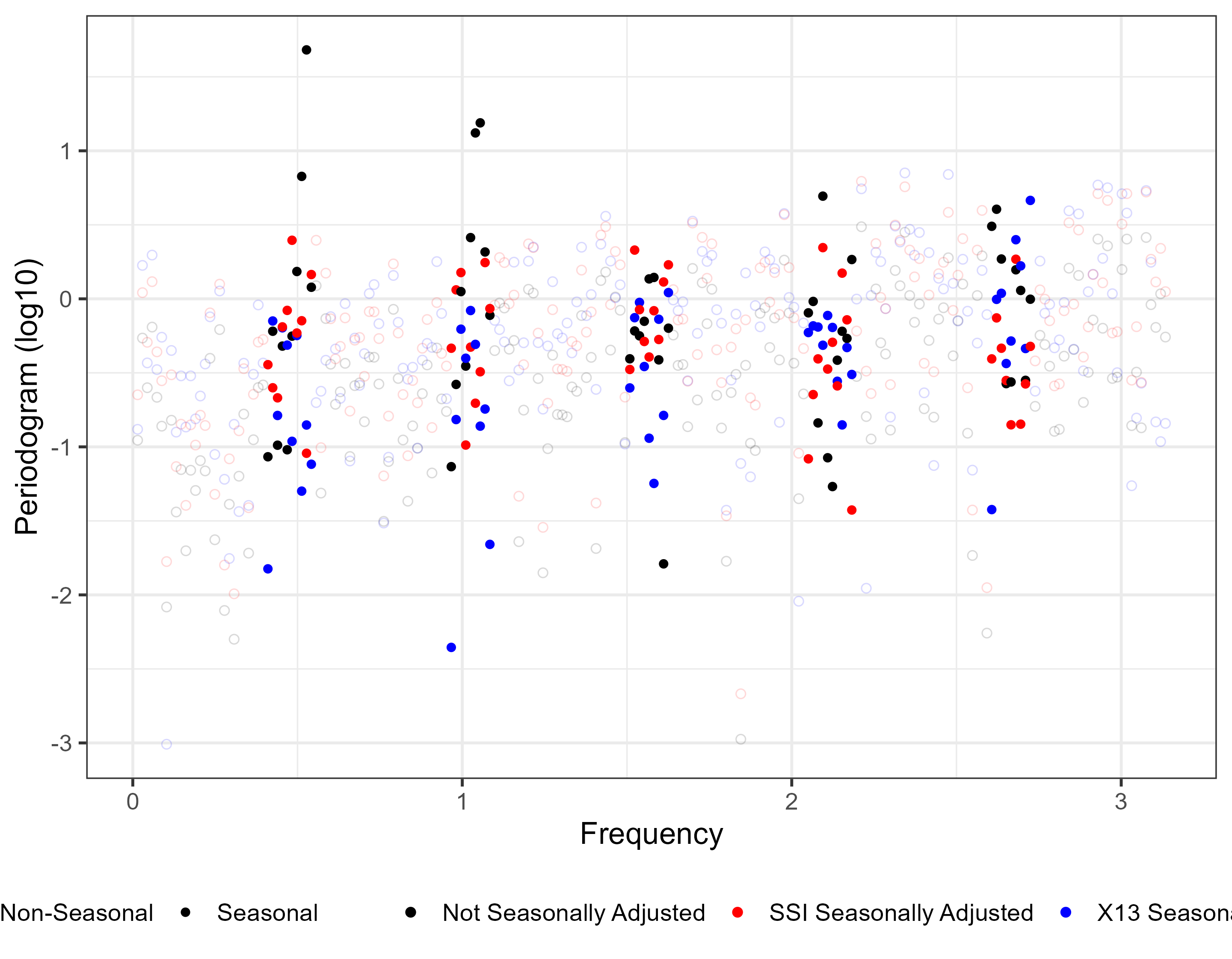
→ SSI ordinates in seasonal bins sit at the non-seasonal floor. X-13’s ordinates dip below the floor — the canonical spectral trough of filter-based methods.

The second housing-starts diagnostic: SSI leaves seasonal-bin ordinates at the non-seasonal floor, while X-13 digs below it — the canonical spectral trough of filter-based adjustment.

SSI surgery — explore

makeSurgery({explore: true})

Genuine freqseas output: all variants and donor draws precomputed in R (R/make_w4_data.R); the head window (first 12 observations) is unadjusted by construction; displayed level totals are forced to the NSA yearly sums at every frame (pro-rata, freqseas::benchmark_totals).

Sandbox over the exported variant grid: switch donor quantile and imputation method, reseed through the precomputed draws to build the uncertainty-band intuition (previous paths remain as gray ghosts until Reset), toggle levels vs log-differences, and compare against the package-default band branch — deterministic, and its post-test honestly fails.

// Unique-id generator in its OWN cell, so the widget factories never reference
// their own name (self-reference is a circular definition in OJS). Copied from
// ar1_spike.qmd.
nextUid = (function () { let n = 0; return () => ++n; })()

// ---------------------------------------------------------------------------
// Widget factories (design doc §5) — one reusable factory per widget, each in
// its own OJS cell, instantiated per-slide with an options object.
//   W4 makeSurgery  — BUILT below; binding spec = w4_spec.md.
//   W3 makeNullDist — BUILT below (slide "The null distribution"): seeded JS
//        Exp(1) draws on the payrolls grid, maxima flash, Δ̂ fills a histogram
//        over the exact Logistic null (freqseas evt.R: standardized ordinates,
//        tau_hat = 1, location log(N1/N0), scale 1 — NOT log-ordinates).
//   W2 makePartition — BUILT below; ONE factory, THREE mounts across the slides
//        "the partition" / "Delta" / "the sample analog", progressively revealing
//        the population object: opts.mode = "bins" (support and colouring only),
//        "sdf" (synthetic closed-form density + population Delta), "sample" (one
//        seeded f*Exp(1) draw + Delta-hat). No data dependency at all — these
//        three slides are population-level pedagogy and deliberately predate the
//        payrolls series. M is shared across the mounts via the partitionM cell.
//        Bin rule mirrors freqseas partition.R (right-closed equal-width bins,
//        Nyquist harmonic included per seas_test).
//        [WAS makeBins, on the payrolls whitened periodogram, until 2026-08-17.]
//   [RETIRED 2026-08-14] makeFourier (W1) — replaced by the manim time→frequency
//        clip figures/time_to_frequency.mp4 (source: Dropbox Misc/frequency_animation).
// Shared rules: hand-drawn SVG, deterministic seeded RNG, rAF loop gated on
// section.present with a max-seconds cap; animations only run over HTTP.
// ---------------------------------------------------------------------------

// W4 data: built by R/make_w4_data.R (contract "coeffs_windowed"). Loaded once,
// shared by both makeSurgery mounts (slide 18 + appendix A10).
// ?v= pins the browser-cache identity to the data schema: bump it whenever
// make_w4_data.R regenerates the file (plain HTTP servers send no Cache-Control,
// and Chrome's heuristic cache will otherwise happily serve a stale copy).
w4data = FileAttachment("data/w4_surgery.json?v=2").json()

// ============================ makeSurgery (W4) ==============================
// Reusable SSI-surgery widget factory per w4_spec.md §4 (ar1_spike pattern:
// per-instance state, hand-drawn SVG, rAF loop gated on section.present).
// opts: { explore: bool }  — explore adds quantile/method/reseed/view/reset.
// All statistics precomputed in R; JS only replays and reconstructs.
// Index conventions (meta.index_convention / meta.coef_convention, R is
// 1-based): JS 0-based i into dlog arrays maps to R t = i+1, so
//   delta_k(i) = Re[(c_re + i·c_im)·e^{i·omega_k·(i+1−t0)}]  for i ≥ t0−1,
// omega_k = 2π·j_k/n_e; levels: loglvl[0] = log_nsa[0], loglvl[m+1] =
// loglvl[m] + dl[m]; the final state SNAPS to the variant's final_dlog_check.
// LEVEL DISPLAYS ARE BENCHMARKED (schema v2, spec §1.5 pro-rata branch): every
// frame forces yearly totals to the NSA sums via meta.benchmark.rule —
// factor_y = year_sums_nsa[y] / Σ level over year y's 12-obs block (JS 0-based
// block y*12..y*12+11) — deterministic accounting arithmetic, the sanctioned
// exception to "no statistics in JS". The snapped state displays the exported
// final_level_bench exactly; the chip shows evt_after_bench.
makeSurgery = function (opts) {
  opts = opts || {};
  const uid = nextUid();
  const explore = !!opts.explore;

  // ---- data unpack -------------------------------------------------------
  const META = w4data.meta, SH = w4data.shared, VS = w4data.variants;
  const T = META.n_dlog, t0 = META.t0, NE = META.n_e, NS = META.n_spec;
  const ALPHA = SH.evt_before.alpha;
  const TG = SH.targets, NT = TG.length;
  const OMG = TG.map(t => 2 * Math.PI * t.j / NE);      // exact phases from j
  const dlog0 = Float64Array.from(SH.dlog_nsa);
  const pgB = SH.pgram_before;
  const lvlNSA = SH.level_nsa, lvlSA = SH.level_x13, dates = SH.dates;
  const logNSA0 = SH.log_nsa[0];
  const dlogSA = new Float64Array(T);
  for (let i = 0; i < T; i++) dlogSA[i] = Math.log(lvlSA[i + 1]) - Math.log(lvlSA[i]);
  const bandV = VS.find(v => v.is_band_default);
  const defV = VS.find(v => v.is_default);
  const bandAfter = pgB.map((p, jj) => p / (bandV.gain_pos[jj] * bandV.gain_pos[jj]));
  const NY = SH.benchmark.n_years, YS = SH.benchmark.year_sums_nsa;   // 87 × 12 = n_obs

  // play order: slow beats = first ordinate of harmonics 1–3, then the rest
  // straight through in exported animation order (additive deltas, so any
  // order reconstructs exactly).
  const firstOfH = [];
  TG.forEach((t, i) => { if (firstOfH[t.harmonic - 1] === undefined) firstOfH[t.harmonic - 1] = i; });
  const slowIdx = firstOfH.slice(0, 3);
  const order = slowIdx.concat(TG.map((_, i) => i).filter(i => slowIdx.indexOf(i) < 0));

  // harmonic bin extents (grid-index runs of the targets) for shading/labels
  const hInfo = [];
  TG.forEach((t, i) => {
    const h = t.harmonic - 1;
    if (!hInfo[h]) hInfo[h] = { label: t.harmonic_label, jmin: t.j, jmax: t.j };
    hInfo[h].jmin = Math.min(hInfo[h].jmin, t.j);
    hInfo[h].jmax = Math.max(hInfo[h].jmax, t.j);
  });

  // ---- reconstruction math ----------------------------------------------
  const applyDelta = (dl, V, k, sign) => {          // O(T): add ordinate k's delta
    const cr = sign * V.c_re[k], ci = sign * V.c_im[k], w = OMG[k];
    const cw = Math.cos(w), sw = Math.sin(w);
    let er = 1, ei = 0;                             // e^{i·w·(i+1-t0)}, i = t0-1 first
    for (let i = t0 - 1; i < T; i++) {
      dl[i] += cr * er - ci * ei;
      const nr = er * cw - ei * sw; ei = er * sw + ei * cw; er = nr;
    }
  };
  const deltaSeries = (V, k) => {                   // the windowed sinusoid alone
    const d = new Float64Array(T);
    applyDelta(d, V, k, 1);
    return d;
  };
  const levelsFrom = dl => {                        // cumulate: log-levels, len T+1
    const L = new Float64Array(T + 1);
    L[0] = logNSA0;
    for (let i = 0; i < T; i++) L[i + 1] = L[i] + dl[i];
    return L;
  };
  const benchLevels = L => {                        // meta.benchmark.rule (pro-rata
    const out = new Float64Array(T + 1);            // per 12-obs year block)
    for (let m = 0; m <= T; m++) out[m] = Math.exp(L[m]);
    for (let y = 0; y < NY; y++) {
      let s = 0; const a = y * 12;
      for (let m = a; m < a + 12; m++) s += out[m];
      const f = YS[y] / s;
      for (let m = a; m < a + 12; m++) out[m] *= f;
    }
    return out;
  };

  // JS self-check (spec §4 / exporter flag): (a) rebuild the default variant's
  // final dlog from coefficients alone, tolerance max(2·coef_final_dev, 1e-6);
  // (b) benchmark the snapped levels via the JS rule and compare to the
  // exported final_level_bench, tolerance 1e-6 RELATIVE (exporter measured
  // 4.87e-9 for this consumer-side mirror).
  let checkFailed = false;
  {
    const test = Float64Array.from(dlog0);
    for (let k = 0; k < NT; k++) applyDelta(test, defV, k, 1);
    let dev = 0;
    for (let i = 0; i < T; i++) dev = Math.max(dev, Math.abs(test[i] - defV.final_dlog_check[i]));
    const tol = Math.max(2 * defV.coef_final_dev, META.validation.js_snap_tolerance);
    if (!(dev <= tol)) {
      checkFailed = true;
      console.error(`makeSurgery[${uid}] self-check FAILED: coefficient reconstruction ` +
                    `dev ${dev.toExponential(3)} > tol ${tol.toExponential(3)}`);
    }
    const bl = benchLevels(levelsFrom(defV.final_dlog_check));
    let rel = 0;
    for (let m = 0; m <= T; m++)
      rel = Math.max(rel, Math.abs(bl[m] - defV.final_level_bench[m]) /
                          Math.abs(defV.final_level_bench[m]));
    if (!(rel <= 1e-6)) {
      checkFailed = true;
      console.error(`makeSurgery[${uid}] self-check FAILED: benchmark mirror rel dev ` +
                    `${rel.toExponential(3)} > 1e-6 vs final_level_bench`);
    }
  }

  // ---- geometry ----------------------------------------------------------
  // H was 772 when the minimap caption lived inside the plot (baseline nB + 26);
  // that caption is HTML now, so the box ends 20 units under the minimap — still
  // clear of the invisible .mhit drag target, which reaches nB + 8 = 744.
  const W = 1700, H = 756, mL = 74, mR = 30;
  const iw = W - mL - mR;
  const pT = 16, pB = 296;                          // periodogram panel
  const tT = 372, tB = 630;                         // time panel
  const nT = 668, nB = 736;                         // minimap
  const xJ = j => mL + (j / NS) * iw;               // grid index -> x (omega scale)

  // log10 power scale: domain covers before + every exported after (band incl.)
  let pLo = Infinity, pHi = -Infinity;
  const eat = v => { if (v > 0) { pLo = Math.min(pLo, v); pHi = Math.max(pHi, v); } };
  pgB.forEach(eat); bandAfter.forEach(eat);
  VS.forEach(v => { if (v.pgram_after) v.pgram_after.forEach(eat); });
  const l10 = Math.log10, pLo10 = l10(pLo) - 0.25, pHi10 = l10(pHi) + 0.25;
  const yP = v => pT + (pHi10 - l10(Math.max(v, 1e-300))) / (pHi10 - pLo10) * (pB - pT);

  // default zoom: 6 years ending the December before the COVID cliff (the
  // cliff stays visible in the full-range minimap; spec §4). The window is
  // MOVABLE: dragging the minimap recenters it (fixed width, display-only).
  // ponytail: fixed 6-year width, drag-to-move only — resize handles only if requested.
  let cliff = 0;
  for (let i = 1; i < T; i++) if (dlog0[i] < dlog0[cliff]) cliff = i;
  const ZW = 71;                                    // window span: 72 monthly obs
  const zmDefault = Math.max(ZW + 1, cliff + 1 - 4) - ZW;
  let zm0 = zmDefault, zm1 = zmDefault + ZW;        // mutable level indices
  const xT = m => mL + ((m - zm0) / ZW) * iw;

  // y domains over the CURRENT zoom window (recomputed on drag so nothing
  // clips): levels = NSA ∪ X-13 ∪ default benchmarked final; dlog likewise
  let lvLo = 0, lvHi = 1, dLo = 0, dHi = 1;
  const computeYDomains = () => {
    lvLo = Infinity; lvHi = -Infinity;
    for (let m = zm0; m <= zm1; m++) {
      lvLo = Math.min(lvLo, lvlNSA[m], lvlSA[m], defV.final_level_bench[m]);
      lvHi = Math.max(lvHi, lvlNSA[m], lvlSA[m], defV.final_level_bench[m]);
    }
    const padL = 0.07 * (lvHi - lvLo);
    lvLo = (lvLo - padL) / 1000; lvHi = (lvHi + padL) / 1000;   // millions
    dLo = Infinity; dHi = -Infinity;
    for (let i = Math.max(0, zm0 - 1); i <= zm1 - 1; i++) {
      dLo = Math.min(dLo, dlog0[i], dlogSA[i]);
      dHi = Math.max(dHi, dlog0[i], dlogSA[i]);
    }
    const padD = 0.1 * (dHi - dLo); dLo -= padD; dHi += padD;
  };
  computeYDomains();
  const yLv = v => tT + (lvHi - v) / (lvHi - lvLo) * (tB - tT);
  const yDl = v => tT + (dHi - v) / (dHi - dLo) * (tB - tT);

  // minimap scales (full range, levels; COVID cliff visible)
  let nLo = Infinity, nHi = -Infinity;
  for (let m = 0; m <= T; m++) { nLo = Math.min(nLo, lvlNSA[m]); nHi = Math.max(nHi, lvlNSA[m]); }
  const xN = m => mL + (m / T) * iw;
  const yN = v => nT + (nHi - v) / (nHi - nLo) * (nB - nT);

  // ---- path builders -----------------------------------------------------
  const P = (x, y) => x.toFixed(1) + " " + y.toFixed(1);
  const zoomPathLevelsRaw = arr => {                // arr = levels in thousands
    let d = "";
    for (let m = zm0; m <= zm1; m++) d += (m === zm0 ? "M" : "L") + P(xT(m), yLv(arr[m] / 1000));
    return d;
  };
  const zoomPathDlog = dl => {
    let d = "";
    const i0 = Math.max(0, zm0 - 1);                // month 0 has no dlog
    for (let i = i0; i <= zm1 - 1; i++)
      d += (i === i0 ? "M" : "L") + P(xT(i + 1), yDl(dl[i]));
    return d;
  };
  const miniPathRaw = arr => {
    let d = "";
    for (let m = 0; m <= T; m += 2) d += (m === 0 ? "M" : "L") + P(xN(m), yN(arr[m]));
    return d;
  };

  // published-series overlays, both domains — zoom-dependent, rebuilt by
  // applyZoom() whenever the window moves (minimap NSA path is zoom-free)
  let pNSAlv = "", pSAlv = "", pNSAdl = "", pSAdl = "";
  const pathNSAmini = miniPathRaw(lvlNSA);

  // ---- formatting helpers ------------------------------------------------
  const statFmt = s => Math.abs(s) >= 10 ? s.toFixed(1) : s.toFixed(2);
  // sup() now serves the SVG log-power decades ONLY: a <tspan dy> pair is the
  // one place a superscript still has to be hand-drawn, because that label is
  // an axis tick inside the plot.
  const sup = (txt, fs) => `<tspan dy="-9" font-size="${fs || 14}">${txt}</tspan>`;
  // KaTeX for the header/footer chrome. The page's math hook (bls_slides.html
  // <head>) only fires on DOMContentLoaded, so OJS-built markup has to call
  // katex itself. Guarded: a dead CDN should cost raw TeX, not the whole widget.
  // ponytail: raw TeX beats a blank slide mid-presentation.
  const kx = t => (typeof katex !== "undefined")
    ? katex.renderToString(t, { throwOnError: false })
    : t;
  // p-value as TeX, replacing pFmt: the readout it feeds is HTML now, and
  // pFmt's <tspan dy="-9"> superscripts only mean anything inside an <svg>.
  const pTeX = p => {
    if (p <= 0) return "p < 10^{-15}";
    if (p < 1e-3) {
      const e = Math.floor(l10(p)), m = (p / Math.pow(10, e)).toFixed(1);
      return `p = ${m} \\times 10^{${e}}`;
    }
    return `p = ${p.toFixed(3)}`;
  };

  // ---- static SVG skeleton ----------------------------------------------
  const root = document.createElement("div");
  root.style.cssText = "width:100%;";

  // seasonal-bin shading + harmonic flash labels
  let shadeS = "", hLabS = "";
  hInfo.forEach((h, i) => {
    const x0 = xJ(h.jmin - 0.5), x1 = Math.min(xJ(h.jmax + 0.5), mL + iw);
    shadeS += `<rect x="${x0.toFixed(1)}" y="${pT}" width="${(x1 - x0).toFixed(1)}" height="${pB - pT}" fill="var(--bea-lblue)" opacity="0.5"/>`;
    hLabS += `<text class="hlab" data-h="${i}" x="${((x0 + x1) / 2).toFixed(1)}" y="${pT + 26}" text-anchor="middle" font-size="24" font-weight="700" fill="var(--bea-blue)" opacity="0">${h.label}</text>`;
  });

  // base periodogram dots (all NS ordinates)
  let baseS = "";
  for (let jj = 0; jj < NS; jj++)
    baseS += `<circle class="pd" cx="${xJ(jj + 1).toFixed(1)}" cy="${yP(pgB[jj]).toFixed(1)}" r="2.2" fill="var(--bea-gray)"/>`;

  // frequency axis ticks at multiples of pi/6
  const fLab = ["0", "π/6", "π/3", "π/2", "2π/3", "5π/6", "π"];
  let fAxS = "";
  for (let i = 0; i <= 6; i++) {
    const x = mL + (i / 6) * iw;
    fAxS += `<line x1="${x}" y1="${pB}" x2="${x}" y2="${pB + 7}" stroke="#999"/>` +
            `<text x="${x}" y="${pB + 30}" text-anchor="middle" font-size="19" fill="#666">${fLab[i]}</text>`;
  }

  // time-panel year ticks (zoom window Januaries) — rebuilt on window move
  const buildTAx = () => {
    let s = "";
    for (let m = zm0; m <= zm1; m++) if (dates[m].slice(5, 7) === "01")
      s += `<line x1="${xT(m).toFixed(1)}" y1="${tB}" x2="${xT(m).toFixed(1)}" y2="${tB + 7}" stroke="#999"/>` +
           `<text x="${xT(m).toFixed(1)}" y="${tB + 30}" text-anchor="start" font-size="19" fill="#666">${dates[m].slice(0, 4)}</text>`;
    return s;
  };

  // y ticks per domain — rebuilt on window move
  const ticksOf = (lo, hi, n) => {
    const span = hi - lo, step = Math.pow(10, Math.floor(l10(span / n)));
    const mult = span / n / step >= 5 ? 5 : span / n / step >= 2 ? 2 : 1;
    const s = mult * step, out = [];
    for (let v = Math.ceil(lo / s) * s; v <= hi + 1e-12; v += s) out.push(v);
    return out;
  };
  const buildLvTicks = () => ticksOf(lvLo, lvHi, 4).map(v =>
    `<line x1="${mL}" y1="${yLv(v).toFixed(1)}" x2="${mL + iw}" y2="${yLv(v).toFixed(1)}" stroke="#eee"/>` +
    `<text x="${mL - 10}" y="${(yLv(v) + 6).toFixed(1)}" text-anchor="end" font-size="19" fill="#666">${v.toFixed(0)}M</text>`).join("");
  const buildDlTicks = () => ticksOf(dLo, dHi, 4).map(v =>
    `<line x1="${mL}" y1="${yDl(v).toFixed(1)}" x2="${mL + iw}" y2="${yDl(v).toFixed(1)}" stroke="#eee"/>` +
    `<text x="${mL - 10}" y="${(yDl(v) + 6).toFixed(1)}" text-anchor="end" font-size="19" fill="#666">${(v * 100).toFixed(1)}%</text>`).join("");
  const pTickS = (() => {
    let s = "";
    for (let e = Math.ceil(pLo10); e <= Math.floor(pHi10); e++) {
      const y = pT + (pHi10 - e) / (pHi10 - pLo10) * (pB - pT);
      s += `<line x1="${mL}" y1="${y.toFixed(1)}" x2="${mL + iw}" y2="${y.toFixed(1)}" stroke="#f0f0f0"/>` +
           `<text x="${mL - 10}" y="${(y + 6).toFixed(1)}" text-anchor="end" font-size="18" fill="#888">10${sup(e, 13)}</text>`;
    }
    return s;
  })();

  const chart = document.createElement("div");
  chart.innerHTML =
`<svg viewBox="0 0 ${W} ${H}" style="width:100%;height:auto;display:block;font-family:inherit;">
  <defs><clipPath id="w4clip${uid}"><rect x="${mL}" y="${tT}" width="${iw}" height="${tB - tT}"/></clipPath></defs>

  <!-- periodogram panel -->
  ${shadeS}${pTickS}
  <line x1="${mL}" y1="${pB}" x2="${mL + iw}" y2="${pB}" stroke="#333" stroke-width="2"/>${fAxS}
  <g class="gbase">${baseS}</g>
  <g class="gpool"></g>
  <line class="thline" x1="${mL}" y1="0" x2="${mL + iw}" y2="0" stroke="var(--bea-gray)" stroke-width="2.5" stroke-dasharray="8 6" opacity="0.55"/>
  <text class="thlab" x="${mL + 10}" y="0" font-size="19" font-style="italic" fill="#666"></text>
  <g class="grings"></g>
  <g class="gtgt"></g>
  <path class="donarc" fill="none" stroke="var(--bea-teal)" stroke-width="3" opacity="0" d=""/>
  <circle class="donflash" r="9" fill="none" stroke="var(--bea-teal)" stroke-width="3.5" opacity="0" cx="-20" cy="-20"/>
  <!-- panel title and the before/after Delta-hat chip are HTML chrome now (see
       the header block below): the chip was a 392x100 white box parked over the
       top-right ordinates, and the title sat in the same band as the harmonic
       flash labels. The flash labels stay — they annotate specific bins. -->
  ${hLabS}

  <!-- time panel -->
  <g class="gtickLv"></g>
  <g class="gtickDl" style="display:none"></g>
  <line x1="${mL}" y1="${tB}" x2="${mL + iw}" y2="${tB}" stroke="#333" stroke-width="2"/>
  <g class="gtax"></g>
  <g clip-path="url(#w4clip${uid})">
    <g class="ghosts"></g>
    <path class="nsaline" fill="none" stroke="var(--bea-gray)" stroke-width="2" opacity="0.8" d=""/>
    <path class="x13line" fill="none" stroke="var(--bea-teal)" stroke-width="2.5" stroke-dasharray="9 6" opacity="0" d=""/>
    <path class="reconline" fill="none" stroke="var(--bea-blue)" stroke-width="3" d=""/>
    <path class="trace" fill="none" stroke="var(--bea-orange)" stroke-width="1.8" opacity="0" d=""/>
  </g>
  <!-- time-panel title, trace label and the NSA/reconstruction/X-13 key are
       HTML chrome now (second header row): the title and trace label overprinted
       the series at the left of the window, and the key crossed whatever the
       reconstruction did at the right of it. -->

  <!-- minimap -->
  <path class="minsa" fill="none" stroke="var(--bea-gray)" stroke-width="1.4" opacity="0.85" d="${pathNSAmini}"/>
  <path class="mrecon" fill="none" stroke="var(--bea-blue)" stroke-width="1.4" d=""/>
  <rect class="mzoom" x="${xN(zm0).toFixed(1)}" y="${nT - 3}" width="${(xN(zm1) - xN(zm0)).toFixed(1)}" height="${nB - nT + 6}" fill="var(--bea-lorange)" opacity="0.4" stroke="var(--bea-orange)" stroke-width="2.5" style="cursor:grab;"/>
  <!-- the minimap caption ("full range … drag …") is the HTML footnote below -->
  <rect class="mhit" x="${mL}" y="${nT - 8}" width="${iw}" height="${nB - nT + 16}" fill="none" pointer-events="all" style="cursor:grab;touch-action:none;"/>
</svg>`;
  const svg = chart.querySelector("svg");
  const $ = sel => svg.querySelector(sel);
  const $$ = sel => Array.prototype.slice.call(svg.querySelectorAll(sel));
  const baseDots = $$(".pd");
  const gPool = $(".gpool"), gRings = $(".grings"), gTgt = $(".gtgt");
  const thLine = $(".thline"), thLab = $(".thlab");
  const donArc = $(".donarc"), donFlash = $(".donflash");
  const hLabs = $$(".hlab");
  const reconLine = $(".reconline"), nsaLine = $(".nsaline"), x13Line = $(".x13line");
  const traceEl = $(".trace");
  const mRecon = $(".mrecon"), ghostsG = $(".ghosts");
  const gTickLv = $(".gtickLv"), gTickDl = $(".gtickDl"), gTax = $(".gtax");
  const mZoomR = $(".mzoom"), mHit = $(".mhit");

  // target overlays (rings at the before-position; dots animate before->after)
  let ringEls = [], tgtEls = [];
  {
    let rS = "", tS = "";
    for (let k = 0; k < NT; k++) {
      const x = xJ(TG[k].j).toFixed(1), y = yP(pgB[TG[k].j - 1]).toFixed(1);
      rS += `<circle cx="${x}" cy="${y}" r="6.5" fill="none" stroke="var(--bea-orange)" stroke-width="2" opacity="0.35"/>`;
      tS += `<circle cx="${x}" cy="${y}" r="3.4" fill="var(--bea-orange)"/>`;
    }
    gRings.innerHTML = rS; gTgt.innerHTML = tS;
    ringEls = Array.prototype.slice.call(gRings.children);
    tgtEls = Array.prototype.slice.call(gTgt.children);
  }

  // ---- header chrome: one row per panel, ABOVE the plot -------------------
  // All of this used to be drawn inside the <svg>, on top of the data it names:
  // the two panel titles at their panels' top-left, the before/after statistic
  // in a white chip box over the highest ordinates, the trace label under the
  // time-panel title, and the series key across the right of the zoom window.
  // Two rows, in panel order (periodogram, then time panel); the minimap's
  // caption became the footnote below the chart. As HTML the readouts also get
  // real KaTeX — the chip wrote Delta-hat as Δ followed by U+0302, which
  // browsers hang up and to the RIGHT of the Δ rather than centred over it.
  const mkHeadRow = () => {
    const d = document.createElement("div");
    d.style.cssText = "display:flex; align-items:baseline; flex-wrap:wrap; " +
                      "gap:1.2em; margin:0 0 .15em;";
    return d;
  };
  const mkTitle = html => {
    const s = document.createElement("span");
    s.style.cssText = "font-weight:700; color:#444; font-size:.92em;";
    s.innerHTML = html;
    return s;
  };

  const headP = mkHeadRow();                          // periodogram panel
  // Plain text, ₁₀ as the precomposed subscript glyph: that is what the partition widget's
  // title does on the neighbouring slide, and unlike the combining hat this
  // character needs no help. KaTeX is reserved for the readouts below.
  headP.append(mkTitle("whitened periodogram (log₁₀ power)"));
  const rBox = document.createElement("div");
  rBox.style.cssText = "margin-left:auto; text-align:right; font-size:.8em; " +
                       "line-height:1.5; white-space:nowrap;";
  const chipB = document.createElement("div");
  chipB.style.color = "var(--bea-orange)";
  chipB.innerHTML = kx(`\\text{before } \\widehat{\\Delta} = ${statFmt(SH.evt_before.statistic)}` +
                       ` \\;\\cdot\\; ${pTeX(SH.evt_before.p)}` +
                       ` \\;\\Rightarrow\\; \\text{reject } H_0`);
  const chipA = document.createElement("div");        // filled by setChipAfter
  rBox.append(chipB, chipA);
  headP.append(rBox);

  const headT = mkHeadRow();                          // time panel
  const tpTitle = mkTitle("");                        // text set by setTitle()
  // The trace label still fades with the sinusoid it names, so render() drives
  // its CSS opacity exactly as it drove the SVG attribute.
  const traceLab = document.createElement("span");
  traceLab.style.cssText = "font-size:.8em; font-style:italic; " +
                           "color:var(--bea-orange); opacity:0; white-space:nowrap;";
  const swatch = (stroke, sw, dash) =>
    `<svg width="30" height="8" style="vertical-align:.08em;">` +
    `<line x1="0" y1="4" x2="30" y2="4" stroke="${stroke}" stroke-width="${sw}"` +
    (dash ? ` stroke-dasharray="${dash}"` : "") + `/></svg>`;
  const legend = document.createElement("div");
  legend.style.cssText = "margin-left:auto; font-size:.8em; color:#666; white-space:nowrap;";
  legend.innerHTML = swatch("var(--bea-gray)", 2.5) + " NSA&ensp;" +
                     swatch("var(--bea-blue)", 3) + " reconstruction";
  const x13Key = document.createElement("span");      // revealed with the X-13 line
  x13Key.style.opacity = "0";
  x13Key.innerHTML = "&ensp;" + swatch("var(--bea-teal)", 2.5, "7 5") + " X-13";
  legend.append(x13Key);
  headT.append(tpTitle, traceLab, legend);

  // ---- controls ----------------------------------------------------------
  const cbar = document.createElement("div");
  cbar.className = "fs-controls";
  const mkBtn = txt => { const b = document.createElement("button"); b.textContent = txt; return b; };
  const mkSel = (lab, opts_) => {
    const w = document.createElement("label");
    const s = document.createElement("span"); s.textContent = lab;
    const sel = document.createElement("select");
    opts_.forEach(o => {
      const e = document.createElement("option");
      e.value = o.value; e.textContent = o.text; sel.appendChild(e);
    });
    w.append(s, sel); return { w, sel };
  };
  const adjB = mkBtn("Adjust"), stepB = mkBtn("Step +1"), skipB = mkBtn("Skip to end");
  const spdW = document.createElement("label");
  spdW.innerHTML = `<span>speed</span>`;
  const spdI = document.createElement("input");
  spdI.type = "range"; spdI.min = "0.25"; spdI.max = "3"; spdI.step = "0.25"; spdI.value = "1";
  const spdO = document.createElement("span"); spdO.className = "cval"; spdO.textContent = "×1";
  spdW.append(spdI, spdO);
  cbar.append(adjB, stepB, skipB, spdW);

  let qSel = null, mSel = null, reseedB = null, drawLab = null, viewB = null, resetB = null;
  if (explore) {
    const qs = mkSel("quantile", SH.donor.quantiles.map(q => ({ value: String(q), text: "q = " + q })));
    qs.sel.value = String(SH.donor.default_quantile);
    const ms = mkSel("method", [
      { value: "bootstrap", text: "bootstrap" },
      { value: "exponential", text: "exponential" },
      { value: "mean", text: "mean" },
      { value: "band", text: "band default (package)" }
    ]);
    qSel = qs.sel; mSel = ms.sel;
    reseedB = mkBtn("Reseed");
    drawLab = document.createElement("span"); drawLab.className = "cval"; drawLab.style.minWidth = "6em";
    viewB = mkBtn("view: levels");
    resetB = mkBtn("Reset");
    cbar.append(qs.w, ms.w, reseedB, drawLab, viewB, resetB);
  }
  if (checkFailed) {
    const warn = document.createElement("span");
    warn.textContent = "⚠ data self-check failed — see console";
    warn.style.cssText = "color:var(--bea-orange);font-weight:700;";
    cbar.append(warn);
  }

  const noteDiv = document.createElement("div");
  noteDiv.style.cssText = "font-size:0.5em;color:#666;line-height:1.35;display:none;margin-top:.2em;";
  // Footnote: the minimap's caption, which used to be SVG text under the strip.
  const foot = document.createElement("div");
  foot.style.cssText = "font-size:.78em; color:#888; line-height:1.4; margin-top:.2em;";
  foot.textContent = `minimap: full range ${dates[0].slice(0, 4)}–${dates[T].slice(0, 4)} — ` +
                     "drag the highlighted window to move the zoom";
  // headT labels the TIME panel, which is the lower half of a single tall SVG —
  // stacked above the figure with headP it read as a second periodogram title.
  // So it rides as an absolute overlay in the empty band between the two panels
  // (periodogram axis labels end ~pB+30 = 326, time panel starts at tT = 372).
  // Same move as the decision diamond on the workflow slide: HTML over SVG,
  // parked in whitespace, so it covers no data and can still carry KaTeX.
  const chartWrap = document.createElement("div");
  chartWrap.style.cssText = "position:relative;";
  headT.style.cssText += "position:absolute; left:0; right:0; margin:0; " +
                         `top:${(336 / H * 100).toFixed(2)}%; pointer-events:none;`;
  chartWrap.append(chart, headT);

  root.append(headP, cbar, chartWrap, foot);
  if (explore) root.append(noteDiv);

  // ---- instance state ----------------------------------------------------
  let V = defV;                       // active variant
  let q = SH.donor.default_quantile, method = "bootstrap", seedIdx = 0;
  let domain = "levels";              // "levels" | "dlog"
  let speed = 1;
  let phase = "idle";                 // idle|setup|beat|cascade|bandstep|closing|done|stepped
  let phaseT = 0, qpos = 0, casStart = 0, casT = 0;
  let setupProg = 0, x13Op = 0, bandU = 0;
  let beatApplied = false, donPulse = 0;
  const flashT = new Float64Array(hInfo.length);
  let lastH = -1;
  const applied = new Uint8Array(NT);
  const dl = Float64Array.from(dlog0);
  let snapped = false;                // after the snap, display final_level_bench exactly
  let dirty = true, activeT = 0;
  let trace = { d: "", op: 0, label: "" };
  const ghosts = [];                  // { lv: dPath, dl: dPath }

  const seedsFor = (q_, m_) => VS.filter(v => !v.is_band_default && v.quantile === q_ &&
    v.method === m_ && v.seed != null).map(v => v.seed).sort((a, b) => a - b);

  const poolInfo = () => SH.donor.by_quantile.find(d => d.quantile === q);

  // durations (seconds, divided by speed at use)
  const D_SETUP = 1.4, D_BEAT = 2.4, D_CASC = 2.6, D_CLOSE = 0.9, D_BAND = 1.8;
  const MAX_ACTIVE = 60;

  // ---- variant / donor visuals ------------------------------------------
  const cyBefore = TG.map(t => yP(pgB[t.j - 1]));
  let cyAfter = [];
  const loadVariant = () => {
    if (method === "band") V = bandV;
    else if (method === "mean") V = VS.find(v => v.quantile === q && v.method === "mean");
    else {
      const seeds = seedsFor(q, method);
      seedIdx = Math.min(seedIdx, seeds.length - 1);
      V = VS.find(v => !v.is_band_default && v.quantile === q && v.method === method &&
                  v.seed === seeds[seedIdx]);
    }
    cyAfter = method === "band" ? TG.map(t => yP(bandAfter[t.j - 1]))
                                : TG.map((t, k) => yP(V.pgram_after[k]));
    if (method !== "band")                            // restore band-morphed base dots
      for (let jj = 0; jj < NS; jj++) baseDots[jj].setAttribute("cy", yP(pgB[jj]).toFixed(1));
    rebuildDonorVisuals();
    if (drawLab) {
      const K = seedsFor(q, method).length;
      drawLab.textContent = method === "band" ? "deterministic"
        : (K ? `draw ${seedIdx + 1} of ${K}` : "deterministic");
    }
    if (reseedB) reseedB.disabled = seedsFor(q, method).length <= 1;
    noteDiv.style.display = (explore && method === "band") ? "block" : "none";
    noteDiv.textContent = method === "band" ? bandV.note : "";
  };

  const rebuildDonorVisuals = () => {
    if (method === "band") {
      gPool.innerHTML = "";
      thLine.setAttribute("opacity", "0"); thLab.textContent = "";
      gRings.setAttribute("opacity", "0");
      return;
    }
    gRings.setAttribute("opacity", "1");
    const info = poolInfo();
    gPool.innerHTML = info.pool.map(j =>
      `<circle cx="${xJ(j).toFixed(1)}" cy="${yP(pgB[j - 1]).toFixed(1)}" r="2.8" fill="var(--bea-teal)" opacity="0.45"/>`).join("");
    const y = yP(info.threshold).toFixed(1);
    thLine.setAttribute("y1", y); thLine.setAttribute("y2", y);
    thLine.setAttribute("opacity", "0.55");
    thLab.setAttribute("y", (Number(y) - 8).toFixed(1));
    thLab.textContent = `donor threshold (q = ${q})`;
  };

  // ---- chip / titles -----------------------------------------------------
  const setChipAfter = on => {
    if (!on) {                                      // HTML now, so colour the element
      chipA.style.color = "#999";
      chipA.innerHTML = kx("\\text{after } \\ldots");
      return;
    }
    const e = V.evt_after_bench, rej = e.p < ALPHA;   // post-test on the BENCHMARKED series
    chipA.style.color = rej ? "var(--bea-orange)" : "var(--bea-blue)";
    chipA.innerHTML = kx(`\\text{after } \\widehat{\\Delta} = ${statFmt(e.statistic)}` +
                         ` \\;\\cdot\\; ${pTeX(e.p)} \\;\\Rightarrow\\; ` +
                         `\\text{${rej ? "reject " : "fail to reject "}} H_0`);
  };
  const setTitle = () => {
    const zr = `${dates[zm0].slice(0, 4)}–${dates[zm1].slice(0, 4)}`;
    tpTitle.textContent = domain === "levels"
      ? `reconstructed levels, millions (totals benchmarked to NSA years) — zoom ${zr}`
      : `reconstructed log-differences (surgery domain, pre-benchmark) — zoom ${zr}`;
  };

  // ---- run control -------------------------------------------------------
  const resetRun = () => {
    dl.set(dlog0); applied.fill(0);
    qpos = 0; casStart = 0; phase = "idle"; phaseT = 0; casT = 0;
    setupProg = 0; x13Op = 0; bandU = 0; activeT = 0; snapped = false;
    trace.op = 0; donPulse = 0; lastH = -1; flashT.fill(0);
    setChipAfter(false); dirty = true;
  };
  const snapFinal = () => { dl.set(V.final_dlog_check); snapped = true; dirty = true; };
  const finishRun = () => {
    snapFinal(); applied.fill(1); qpos = NT;
    x13Op = 1; bandU = 1; setupProg = 1;
    setChipAfter(true); phase = "done";
  };
  const applyOrd = k => {
    applyDelta(dl, V, k, 1); applied[k] = 1; dirty = true;
    const h = TG[k].harmonic - 1;
    if (h !== lastH) { flashT[h] = 0.8; lastH = h; }
  };
  const beginNext = () => {
    if (qpos >= NT) { phase = "closing"; phaseT = 0; snapFinal(); setChipAfter(true); return; }
    if (qpos < slowIdx.length) { phase = "beat"; phaseT = 0; beatApplied = false; }
    else { phase = "cascade"; casStart = qpos; casT = 0; }
  };
  const startRun = () => {
    resetRun();
    phase = "setup"; phaseT = 0;
  };
  const makeTrace = k => {
    const del = deltaSeries(V, k);
    let amp = 0;
    const i0 = Math.max(0, zm0 - 1);
    for (let i = i0; i <= zm1 - 1; i++) amp = Math.max(amp, Math.abs(del[i]));
    const mid = (tT + tB) / 2, px = amp > 0 ? 34 / amp : 0;
    let d = "";
    for (let i = i0; i <= zm1 - 1; i++)
      d += (i === i0 ? "M" : "L") + P(xT(i + 1), mid - del[i] * px);
    trace.d = d; trace.label = `extracted ${TG[k].harmonic_label} component (rescaled)`;
  };

  // ---- ghosts ------------------------------------------------------------
  const pushGhost = () => {
    if (phase !== "done") return;                   // done => snapped: exact exported series
    ghosts.push({ lv: V.final_level_bench, dl: Float64Array.from(dl) });   // data, not
    if (ghosts.length > 12) ghosts.shift();         // paths — survives zoom-window moves
    renderGhosts();
  };
  const renderGhosts = () => {
    ghostsG.innerHTML = ghosts.map(g =>
      `<path fill="none" stroke="#b9bdbd" stroke-width="1.4" opacity="0.65" d="${
        domain === "levels" ? zoomPathLevelsRaw(g.lv) : zoomPathDlog(g.dl)}"/>`).join("");
  };
  const clearGhosts = () => { ghosts.length = 0; renderGhosts(); };

  // ---- render ------------------------------------------------------------
  const ease = u => u < 0.5 ? 2 * u * u : 1 - 2 * (1 - u) * (1 - u);
  function render(dt) {
    // setup-flash intensity
    const s = setupProg;
    ringEls.forEach((r, k) => {
      r.setAttribute("opacity", applied[k] ? "0.12" : String(0.35 + 0.55 * s));
    });
    gPool.setAttribute("opacity", String(0.6 + 0.4 * s + donPulse * 0.4));
    thLine.setAttribute("stroke-width", String(2.5 + 1.2 * s));

    // target dots
    for (let k = 0; k < NT; k++) {
      const el = tgtEls[k];
      let cy;
      if (applied[k]) { cy = cyAfter[k]; el.setAttribute("fill", "var(--bea-blue)"); }
      else if (phase === "beat" && order[qpos] === k) {
        const u = Math.max(0, Math.min(1, (phaseT / (D_BEAT / speed) - 0.3) / 0.3));
        cy = cyBefore[k] + (cyAfter[k] - cyBefore[k]) * ease(u);
        el.setAttribute("fill", "var(--bea-orange)");
      } else if (phase === "bandstep") {
        cy = cyBefore[k] + (cyAfter[k] - cyBefore[k]) * ease(bandU);
        el.setAttribute("fill", bandU > 0.5 ? "var(--bea-blue)" : "var(--bea-orange)");
      } else { cy = cyBefore[k]; el.setAttribute("fill", "var(--bea-orange)"); }
      el.setAttribute("cy", cy.toFixed(1));
    }
    // band morph moves every base ordinate (deterministic gain division)
    if (method === "band") {
      const u = phase === "done" ? 1 : ease(bandU);
      for (let jj = 0; jj < NS; jj++) {
        const y0 = yP(pgB[jj]), y1 = yP(bandAfter[jj]);
        baseDots[jj].setAttribute("cy", (y0 + (y1 - y0) * u).toFixed(1));
      }
    }

    // harmonic flash labels
    for (let h = 0; h < hInfo.length; h++) {
      if (flashT[h] > 0) flashT[h] = Math.max(0, flashT[h] - dt);
      hLabs[h].setAttribute("opacity", String(Math.min(1, flashT[h] / 0.3)));
    }

    // donor flash + arc (slow beats; honest donor_j exists for bootstrap only)
    if (phase === "beat" && V.donor_j) {
      const k = order[qpos], dj = V.donor_j[k];
      const u = phaseT / (D_BEAT / speed);
      const op = u < 0.3 ? Math.min(1, u / 0.08) : Math.max(0, 1 - (u - 0.3) / 0.15);
      const dx = xJ(dj), dy = yP(pgB[dj - 1]), tx = xJ(TG[k].j), ty = cyAfter[k];
      donFlash.setAttribute("cx", dx.toFixed(1)); donFlash.setAttribute("cy", dy.toFixed(1));
      donFlash.setAttribute("opacity", String(op));
      donArc.setAttribute("d", `M ${P(dx, dy)} Q ${P((dx + tx) / 2, Math.min(dy, ty) - 70)} ${P(tx, ty)}`);
      donArc.setAttribute("opacity", String(op * 0.8));
    } else { donFlash.setAttribute("opacity", "0"); donArc.setAttribute("opacity", "0"); }
    if (donPulse > 0) donPulse = Math.max(0, donPulse - dt);

    // trace (the label is HTML chrome now, so it fades via CSS opacity)
    traceEl.setAttribute("d", trace.d);
    traceEl.setAttribute("opacity", String(trace.op));
    traceLab.textContent = trace.label;
    traceLab.style.opacity = String(trace.op);

    // reconstruction paths — LEVEL displays are always benchmarked; the
    // snapped state shows the exported final_level_bench exactly
    if (dirty) {
      const bl = snapped ? V.final_level_bench : benchLevels(levelsFrom(dl));
      if (domain === "levels") reconLine.setAttribute("d", zoomPathLevelsRaw(bl));
      else reconLine.setAttribute("d", zoomPathDlog(dl));   // surgery domain, pre-benchmark
      mRecon.setAttribute("d", miniPathRaw(bl));
      dirty = false;
    }
    x13Line.setAttribute("opacity", String(x13Op));
    x13Key.style.opacity = String(x13Op);           // key is HTML chrome now
  }

  const setDomain = dom => {
    domain = dom;
    gTickLv.style.display = dom === "levels" ? "" : "none";
    gTickDl.style.display = dom === "dlog" ? "" : "none";
    nsaLine.setAttribute("d", dom === "levels" ? pNSAlv : pNSAdl);
    x13Line.setAttribute("d", dom === "levels" ? pSAlv : pSAdl);
    if (viewB) viewB.textContent = "view: " + (dom === "levels" ? "levels" : "log-diff (pre-benchmark)");
    setTitle(); renderGhosts(); dirty = true;
  };

  // rebuild everything the zoom window touches (scales, ticks, axis, published
  // overlays, minimap indicator, ghosts, title); recon redraws via dirty
  const applyZoom = () => {
    computeYDomains();
    gTickLv.innerHTML = buildLvTicks();
    gTickDl.innerHTML = buildDlTicks();
    gTax.innerHTML = buildTAx();
    pNSAlv = zoomPathLevelsRaw(lvlNSA); pSAlv = zoomPathLevelsRaw(lvlSA);
    pNSAdl = zoomPathDlog(dlog0);       pSAdl = zoomPathDlog(dlogSA);
    nsaLine.setAttribute("d", domain === "levels" ? pNSAlv : pNSAdl);
    x13Line.setAttribute("d", domain === "levels" ? pSAlv : pSAdl);
    mZoomR.setAttribute("x", xN(zm0).toFixed(1));
    mZoomR.setAttribute("width", (xN(zm1) - xN(zm0)).toFixed(1));
    if (phase === "beat" && trace.d !== "") makeTrace(order[qpos]);  // re-project
    setTitle(); renderGhosts(); dirty = true;
  };

  // minimap drag: recenter the fixed-width window at the pointer (clamped)
  let mapDrag = false;
  const zoomToPointer = e => {
    const r = svg.getBoundingClientRect();
    const xv = (e.clientX - r.left) / r.width * W;             // viewBox coords
    const mm = Math.round((xv - mL) / iw * T);                 // month at pointer
    const nz = Math.max(0, Math.min(T - ZW, mm - (ZW >> 1)));
    if (nz !== zm0) { zm0 = nz; zm1 = zm0 + ZW; applyZoom(); }
  };
  mHit.addEventListener("pointerdown", e => {
    mapDrag = true;
    try { mHit.setPointerCapture(e.pointerId); } catch (_) { /* synthetic pointer */ }
    mHit.style.cursor = "grabbing"; mZoomR.style.cursor = "grabbing";
    e.preventDefault(); e.stopPropagation();
    zoomToPointer(e);
  });
  mHit.addEventListener("pointermove", e => { if (mapDrag) zoomToPointer(e); });
  const endMapDrag = () => {
    mapDrag = false; mHit.style.cursor = "grab"; mZoomR.style.cursor = "grab";
  };
  mHit.addEventListener("pointerup", endMapDrag);
  mHit.addEventListener("pointercancel", endMapDrag);

  // ---- state machine -----------------------------------------------------
  function advance(dt) {
    if (phase === "idle" || phase === "done" || phase === "stepped") return;
    activeT += dt;
    if (activeT > MAX_ACTIVE) { finishRun(); return; }
    phaseT += dt;
    if (phase === "setup") {
      setupProg = Math.min(1, phaseT / (D_SETUP / speed));
      if (setupProg >= 1) {
        if (method === "band") { phase = "bandstep"; phaseT = 0; }
        else beginNext();
      }
    } else if (phase === "bandstep") {
      bandU = Math.min(1, phaseT / (D_BAND / speed));
      // visual morph of the recon toward the deterministic final state
      const u = ease(bandU);
      for (let i = 0; i < T; i++) dl[i] = dlog0[i] + (V.final_dlog_check[i] - dlog0[i]) * u;
      dirty = true;
      if (bandU >= 1) { phase = "closing"; phaseT = 0; snapFinal(); setChipAfter(true); }
    } else if (phase === "beat") {
      const u = phaseT / (D_BEAT / speed), k = order[qpos];
      if (!V.donor_j && u < 0.3) donPulse = 0.5;    // no drawn donor: pool glow instead
      if (u >= 0.3 && trace.d === "") makeTrace(k);
      if (u >= 0.6 && !beatApplied) { applyOrd(k); beatApplied = true; }
      trace.op = u < 0.3 ? 0 : u < 0.5 ? (u - 0.3) / 0.2 : u < 0.7 ? 1 : Math.max(0, (1 - u) / 0.3);
      if (u >= 1) { trace.d = ""; trace.op = 0; qpos++; beginNext(); }
    } else if (phase === "cascade") {
      casT += dt;
      const want = casStart + Math.floor((casT / (D_CASC / speed)) * (NT - casStart));
      while (qpos < Math.min(want, NT)) { applyOrd(order[qpos]); qpos++; }
      if (qpos >= NT) { phase = "closing"; phaseT = 0; snapFinal(); setChipAfter(true); }
    } else if (phase === "closing") {
      x13Op = Math.min(1, phaseT / (D_CLOSE / speed));
      if (x13Op >= 1) phase = "done";
    }
  }

  // ---- wire controls -----------------------------------------------------
  adjB.onclick = () => {
    if (phase === "stepped") { setupProg = 1; beginNext(); }
    else startRun();
  };
  stepB.onclick = () => {
    if (phase === "done" || phase === "closing" || qpos >= NT) return;
    if (method === "band") { finishRun(); return; }    // single-step transformation
    if (phase === "idle") resetRun();
    setupProg = 1;
    trace.d = ""; trace.op = 0;
    if (phase === "beat" && beatApplied) qpos++;       // close the half-done beat
    else { applyOrd(order[qpos]); qpos++; donPulse = 0.6; }
    if (qpos >= NT) { snapFinal(); setChipAfter(true); x13Op = 1; phase = "done"; }
    else phase = "stepped";
  };
  skipB.onclick = () => finishRun();
  spdI.oninput = () => { speed = +spdI.value; spdO.textContent = "×" + speed; };

  const refreshDisabled = () => {
    if (!explore) return;
    Array.prototype.forEach.call(qSel.options, o => {
      const qq = Number(o.value);
      o.disabled = method === "band" ? true
        : method === "exponential" ? seedsFor(qq, "exponential").length === 0
        : false;
    });
    Array.prototype.forEach.call(mSel.options, o => {
      o.disabled = o.value === "exponential" ? seedsFor(q, "exponential").length === 0 : false;
    });
    qSel.disabled = method === "band";
  };
  if (explore) {
    qSel.onchange = () => { q = Number(qSel.value); seedIdx = 0; loadVariant(); refreshDisabled(); resetRun(); };
    mSel.onchange = () => { method = mSel.value; seedIdx = 0; loadVariant(); refreshDisabled(); resetRun(); };
    reseedB.onclick = () => {
      pushGhost();                                    // keep the previous path
      const K = seedsFor(q, method).length;
      seedIdx = (seedIdx + 1) % K;
      loadVariant(); resetRun(); startRun();          // re-arm + replay
    };
    viewB.onclick = () => setDomain(domain === "levels" ? "dlog" : "levels");
    resetB.onclick = () => {
      clearGhosts();
      if (zm0 !== zmDefault) { zm0 = zmDefault; zm1 = zmDefault + ZW; applyZoom(); }
      resetRun();
    };
  }

  // ---- start -------------------------------------------------------------
  loadVariant(); refreshDisabled(); applyZoom(); setDomain("levels"); resetRun(); render(0);

  let last = null, prevOn = false;
  function tick(now) {
    if (!document.contains(root)) return;             // orphaned after re-render
    if (last === null) last = now;
    const dt = Math.min(0.1, (now - last) / 1000);
    last = now;
    const onSlide = !!root.closest("section.present");
    if (onSlide && !prevOn) { resetRun(); render(0); }  // fresh arm on slide entry
    prevOn = onSlide;
    if (onSlide) { advance(dt); render(dt); }
    requestAnimationFrame(tick);
  }
  requestAnimationFrame(tick);

  return root;
}

// ============================ makeNullDist (W3) =============================
// Null-distribution animation for slide "The null distribution". Repeated
// draws of N1+N0 i.i.d. Exp(1) ordinates on the REAL payrolls whitened grid
// (n_spec = 516; seasonal positions = the M = 19 partition J1 set, i.e. the
// w4data targets), maxima flash, and Delta = max_J1 - max_J0 (plain
// standardized-ordinate difference — freqseas evt.R/seas_test.R convention,
// tau_hat = 1) drops into a histogram over the exact Logistic null
// Logistic(log(N1/N0), 1). Seeded mulberry32; design doc sanctions JS draws
// for this widget. No statistics beyond the sanctioned simulation arithmetic.
makeNullDist = function (opts) {
  opts = opts || {};
  const uid = nextUid();
  const SH = w4data.shared;
  const NS = SH.pgram_before.length;               // 516 positive ordinates
  const seasJ = SH.targets.map(t => t.j);          // J1 at the payrolls default M = 19
  const isSeas = new Uint8Array(NS + 1);
  seasJ.forEach(j => { isSeas[j] = 1; });
  const N1 = seasJ.length, N0 = NS - N1;           // 165 / 351
  const MU = Math.log(N1 / N0);                    // Logistic location, tau_hat = 1
  const CRIT = MU + Math.log(0.95 / 0.05);         // qlogis(.95, MU, 1)
  const seed = opts.seed || 24601;
  const maxActive = 120, maxDraws = 50000;

  // cross-check the parameterization against the exporter's test output
  let checkFailed = false;
  if (Math.abs(CRIT - SH.evt_before.critical) > 1e-6) {
    checkFailed = true;
    console.error(`makeNullDist[${uid}] null-parameterization check FAILED: ` +
                  `computed c=${CRIT} vs exported ${SH.evt_before.critical}`);
  }

  // seasonal bins of the M = 19 partition, for the shading strips
  const M19 = 19;
  const seasBins = [1, 2, 3, 4, 5, 6].map(k => Math.ceil(k * M19 / 6));

  // ---- geometry ----------------------------------------------------------
  // H was 432 while the methods note sat on the y = H - 6 baseline inside the
  // plot. That note is HTML now, so the box stops 22 units under the lowest
  // axis label (the mu tick at rB + 48 = 378) — enough that descenders on the
  // pi/3, 2pi/3 frequency labels still clear the edge.
  const W = 1700, H = 400;
  const lL = 64, lR = 780, lT = 16, lB = 330;      // left: one draw of ordinates
  const rL = 856, rR = 1666, rT = 16, rB = 330;    // right: Delta histogram
  const VMAX = 12;                                  // left y clamp (visual only)
  const xO = j => lL + (j / NS) * (lR - lL);
  const yO = v => lB - (Math.min(v, VMAX) / VMAX) * (lB - lT);
  const DLO = -8, DHI = 10, NB = 36, BW = (DHI - DLO) / NB;
  const xD = d => rL + ((d - DLO) / (DHI - DLO)) * (rR - rL);
  const DMAX = 0.32;                                // density axis top
  const yD = v => rB - (Math.min(v, DMAX) / DMAX) * (rB - rT);
  const dlogis = x => { const e = Math.exp(-(x - MU)); return e / ((1 + e) * (1 + e)); };

  // ---- RNG (mulberry32) + one replication --------------------------------
  let a = seed >>> 0;
  const unif = () => {
    a = (a + 0x6D2B79F5) >>> 0;
    let t = a;
    t = Math.imul(t ^ (t >>> 15), t | 1);
    t ^= t + Math.imul(t ^ (t >>> 7), t | 61);
    return ((t ^ (t >>> 14)) >>> 0) / 4294967296;
  };
  const vals = new Float64Array(NS + 1);
  let mx1 = 0, mx0 = 0, j1 = 0, j0 = 0, haveDraw = false;
  const drawOnce = () => {
    mx1 = -1; mx0 = -1;
    for (let j = 1; j <= NS; j++) {
      const v = -Math.log(1 - unif());              // Exp(1)
      vals[j] = v;
      if (isSeas[j]) { if (v > mx1) { mx1 = v; j1 = j; } }
      else if (v > mx0) { mx0 = v; j0 = j; }
    }
    haveDraw = true;
    return mx1 - mx0;
  };

  // ---- histogram state ---------------------------------------------------
  const counts = new Int32Array(NB);
  let nDraws = 0, nRej = 0;
  const record = d => {
    const b = Math.max(0, Math.min(NB - 1, Math.floor((d - DLO) / BW)));
    counts[b]++; nDraws++;
    if (d > CRIT) nRej++;
  };

  // ---- static SVG --------------------------------------------------------
  const root = document.createElement("div");
  root.style.cssText = "width:100%;";
  let shadeS = "";
  seasBins.forEach(m => {
    const x0 = xO((m - 1) * NS / M19), x1 = xO(m * NS / M19);
    shadeS += `<rect x="${x0.toFixed(1)}" y="${lT}" width="${(x1 - x0).toFixed(1)}" height="${lB - lT}" fill="var(--bea-lblue)" opacity="0.5"/>`;
  });
  let dotS = "";
  for (let j = 1; j <= NS; j++)
    dotS += `<circle cx="${xO(j).toFixed(1)}" cy="${lB}" r="2.1" fill="${isSeas[j] ? "var(--bea-orange)" : "var(--bea-gray)"}"/>`;
  const fLab = ["0", "π/6", "π/3", "π/2", "2π/3", "5π/6", "π"];
  let lAx = "";
  for (let i = 0; i <= 6; i++) {
    const x = lL + (i / 6) * (lR - lL);
    lAx += `<line x1="${x}" y1="${lB}" x2="${x}" y2="${lB + 7}" stroke="#999"/>` +
           `<text x="${x}" y="${lB + 30}" text-anchor="middle" font-size="19" fill="#666">${fLab[i]}</text>`;
  }
  let lyAx = "";
  for (let v = 0; v <= VMAX; v += 4)
    lyAx += `<line x1="${lL}" y1="${yO(v).toFixed(1)}" x2="${lR}" y2="${yO(v).toFixed(1)}" stroke="#f0f0f0"/>` +
            `<text x="${lL - 10}" y="${(yO(v) + 6).toFixed(1)}" text-anchor="end" font-size="18" fill="#888">${v}</text>`;
  // Logistic pdf + shaded rejection tail (precomputed)
  let pdfS = "", tailS = `M ${xD(CRIT).toFixed(1)} ${rB}`;
  for (let x = DLO; x <= DHI + 1e-9; x += 0.15) {
    pdfS += (pdfS === "" ? "M" : "L") + `${xD(x).toFixed(1)} ${yD(dlogis(x)).toFixed(1)} `;
    if (x >= CRIT) tailS += ` L ${xD(x).toFixed(1)} ${yD(dlogis(x)).toFixed(1)}`;
  }
  tailS += ` L ${xD(DHI).toFixed(1)} ${rB} Z`;
  let rAx = "";
  [-8, -4, 0, 4, 8].forEach(v => {
    rAx += `<line x1="${xD(v).toFixed(1)}" y1="${rB}" x2="${xD(v).toFixed(1)}" y2="${rB + 7}" stroke="#999"/>` +
           `<text x="${xD(v).toFixed(1)}" y="${rB + 30}" text-anchor="middle" font-size="19" fill="#666">${v}</text>`;
  });
  let barS = "";
  for (let b = 0; b < NB; b++)
    barS += `<rect x="${(xD(DLO + b * BW) + 0.5).toFixed(1)}" y="${rB}" width="${((rR - rL) / NB - 1).toFixed(1)}" height="0" fill="var(--bea-mblue)" opacity="0.75"/>`;

  const chart = document.createElement("div");
  chart.innerHTML =
`<svg viewBox="0 0 ${W} ${H}" style="width:100%;height:auto;display:block;font-family:inherit;">
  ${shadeS}${lyAx}
  <line x1="${lL}" y1="${lB}" x2="${lR}" y2="${lB}" stroke="#333" stroke-width="2"/>${lAx}
  <g class="gdots" opacity="0">${dotS}</g>
  <line class="mx1line" x1="${lL}" x2="${lR}" y1="-9" y2="-9" stroke="var(--bea-orange)" stroke-width="2" stroke-dasharray="8 6" opacity="0"/>
  <line class="mx0line" x1="${lL}" x2="${lR}" y1="-9" y2="-9" stroke="#555" stroke-width="2" stroke-dasharray="8 6" opacity="0"/>
  <circle class="mx1ring" r="7" fill="none" stroke="var(--bea-orange)" stroke-width="3" opacity="0" cx="-9" cy="-9"/>
  <circle class="mx0ring" r="7" fill="none" stroke="#333" stroke-width="3" opacity="0" cx="-9" cy="-9"/>
  <!-- panel titles and the Delta-hat readout are HTML chrome now (header row
       above the plot): the readout floated over this panel's top-right corner
       and both titles sat in the band the tallest ordinates reach. -->

  <path d="${tailS}" fill="var(--bea-lorange)" opacity="0.85"/>
  <g class="gbars">${barS}</g>
  <path d="${pdfS}" fill="none" stroke="var(--bea-blue)" stroke-width="3.5"/>
  <line x1="${xD(CRIT).toFixed(1)}" y1="${rB}" x2="${xD(CRIT).toFixed(1)}" y2="${rT + 40}" stroke="var(--bea-orange)" stroke-width="2.5" stroke-dasharray="8 6"/>
  <text x="${xD(CRIT).toFixed(1)}" y="${rB + 30}" text-anchor="middle" font-size="19" fill="var(--bea-orange)">c₀.₀₅</text>
  <line x1="${xD(MU).toFixed(1)}" y1="${rB}" x2="${xD(MU).toFixed(1)}" y2="${rB + 7}" stroke="#999"/>
  <text x="${xD(MU).toFixed(1)}" y="${rB + 48}" text-anchor="middle" font-size="19" font-style="italic" fill="#666">μ</text>
  <line x1="${rL}" y1="${rB}" x2="${rR}" y2="${rB}" stroke="#333" stroke-width="2"/>${rAx}
  <circle class="dropdot" r="6" fill="var(--bea-blue)" opacity="0" cx="-9" cy="-9"/>
  <!-- draw counter and the methods note are HTML chrome too (the note used to
       be SVG text on the y = H - 6 baseline, which set the viewBox height) -->
</svg>`;
  const svg = chart.querySelector("svg");
  const $ = s => svg.querySelector(s);
  const dotsG = $(".gdots");
  const dotEls = Array.prototype.slice.call(dotsG.children);
  const mx1L = $(".mx1line"), mx0L = $(".mx0line");
  const mx1R = $(".mx1ring"), mx0R = $(".mx0ring");
  const dropDot = $(".dropdot");
  const barEls = Array.prototype.slice.call($(".gbars").children);

  // ---- header chrome: one title + readout per panel, ABOVE the plots ------
  // Both panel titles, the per-draw statistic and the draw counter used to be
  // SVG <text> inside the plots: the titles sat in the band the tallest
  // ordinates reach, and the two readouts floated over each panel's top-right
  // corner. One centred title over a two-panel figure would not say which panel
  // it names, so the header is split into two blocks whose offsets and widths
  // track the panels' own viewBox extents (lL..lR and rL..rR of W) — each block
  // carries its panel's title on the left and that panel's live readout right.
  // HTML also buys real KaTeX, which is why the labels moved at all: they wrote
  // Delta-hat as Δ followed by U+0302, and browsers hang that caret up and to
  // the RIGHT of the Δ instead of centring it over the glyph.
  const kx = t => (typeof katex !== "undefined")
    ? katex.renderToString(t, { throwOnError: false })
    : t;                                             // ponytail: raw TeX beats a dead widget
  const pct = u => (100 * u / W).toFixed(2) + "%";
  const mkHalf = (indent, span) => {
    const d = document.createElement("div");
    d.style.cssText = `flex:0 0 ${pct(span)}; margin-left:${pct(indent)}; ` +
                      "display:flex; align-items:baseline; gap:.8em;";
    return d;
  };
  const mkTitle = html => {
    const s = document.createElement("span");
    s.style.cssText = "font-weight:700; color:#444; font-size:.92em;";
    s.innerHTML = html;
    return s;
  };
  const mkReadout = () => {
    const d = document.createElement("div");
    d.style.cssText = "margin-left:auto; text-align:right; font-size:.8em; " +
                      "line-height:1.5; white-space:nowrap; color:#333;";
    return d;
  };
  const head = document.createElement("div");
  head.style.cssText = "display:flex; align-items:flex-start; margin:0 0 .15em;";
  const halfL = mkHalf(lL, lR - lL), halfR = mkHalf(rL - lR, rR - rL);
  const dLab = mkReadout();                          // this draw's statistic
  dLab.style.opacity = "0";                          // render() fades it with the flash
  let dLabTxt = "";                                  // memo: see render()
  halfL.append(mkTitle("one draw: 516 Exp(1) ordinates on the payrolls grid (M = 19)"), dLab);
  const counter = mkReadout();
  halfR.append(mkTitle(kx("\\widehat{\\Delta}") + " across draws vs Logistic(" +
                       kx("\\log(N_1/N_0)") + ", 1)"), counter);
  head.append(halfL, halfR);

  // ---- controls ----------------------------------------------------------
  const cbar = document.createElement("div");
  cbar.className = "fs-controls";
  const playB = document.createElement("button");
  const stepB = document.createElement("button"); stepB.textContent = "Step +1";
  const resetB = document.createElement("button"); resetB.textContent = "Reset";
  const spdW = document.createElement("label");
  spdW.innerHTML = "<span>speed</span>";
  const spdI = document.createElement("input");
  spdI.type = "range"; spdI.min = "0"; spdI.max = "10"; spdI.step = "1"; spdI.value = "2";
  const spdO = document.createElement("span"); spdO.className = "cval"; spdO.style.minWidth = "4.5em";
  spdW.append(spdI, spdO);
  cbar.append(playB, stepB, spdW, resetB);
  if (checkFailed) {
    const warn = document.createElement("span");
    warn.textContent = "⚠ null-parameterization check failed — see console";
    warn.style.cssText = "color:var(--bea-orange);font-weight:700;";
    cbar.append(warn);
  }
  // Methods note: was SVG text on the y = H - 6 baseline, i.e. inside the box.
  const foot = document.createElement("div");
  foot.style.cssText = "font-size:.78em; color:#888; line-height:1.4; margin-top:.2em;";
  foot.innerHTML =
    "simulated in-browser (seeded, deterministic) · " +
    kx(`N_1 = ${N1}`) + ", " + kx(`N_0 = ${N0}`) +
    " from the payrolls default partition · statistic on the " +
    "standardized-ordinate scale (" + kx("\\widehat{\\tau} = 1") + ")";
  root.append(head, cbar, chart, foot);

  // speed detents: draws per second (beat mode through 2/s, batch above)
  const SPD = [0.5, 1, 2, 5, 10, 25, 50, 100, 250, 1000, 5000];
  let speed = SPD[+spdI.value];
  let playing = true, beatT = 0, pending = null, activeT = 0, acc = 0;
  const setPlaying = p => { playing = p; playB.textContent = p ? "⏸ Pause" : "▶ Play"; };
  const fmtPct = x => (100 * x).toFixed(1) + "%";

  const reset = () => {
    a = seed >>> 0; counts.fill(0); nDraws = 0; nRej = 0;
    beatT = 0; pending = null; activeT = 0; acc = 0; haveDraw = false;
  };

  // ---- render ------------------------------------------------------------
  function render() {
    const beat = speed <= 2;
    const dur = 1 / speed;
    const u = beat ? Math.min(1, beatT / dur) : 1;
    // left: dots of the current draw
    if (haveDraw) {
      dotsG.setAttribute("opacity", beat ? String(Math.min(1, u / 0.3)) : "1");
      for (let j = 1; j <= NS; j++) dotEls[j - 1].setAttribute("cy", yO(vals[j]).toFixed(1));
    } else dotsG.setAttribute("opacity", "0");
    // maxima flash
    const fl = haveDraw && (!beat || u >= 0.3) ? 1 : 0;
    const y1 = yO(mx1), y0 = yO(mx0);
    mx1L.setAttribute("y1", y1.toFixed(1)); mx1L.setAttribute("y2", y1.toFixed(1));
    mx0L.setAttribute("y1", y0.toFixed(1)); mx0L.setAttribute("y2", y0.toFixed(1));
    mx1L.setAttribute("opacity", String(fl * 0.9)); mx0L.setAttribute("opacity", String(fl * 0.9));
    mx1R.setAttribute("cx", xO(j1).toFixed(1)); mx1R.setAttribute("cy", y1.toFixed(1));
    mx0R.setAttribute("cx", xO(j0).toFixed(1)); mx0R.setAttribute("cy", y0.toFixed(1));
    mx1R.setAttribute("opacity", String(fl)); mx0R.setAttribute("opacity", String(fl));
    // dLab is HTML/KaTeX now, so only re-render when the shown value moves:
    // katex.renderToString every frame would be waste. Batch mode does change
    // it every frame, but the 516-dot sweep above already dominates that.
    if (fl) {
      const s = (mx1 - mx0).toFixed(2);
      if (s !== dLabTxt) { dLabTxt = s; dLab.innerHTML = kx(`\\widehat{\\Delta} = ${s}`); }
    }
    dLab.style.opacity = String(fl);
    // drop marker
    if (pending !== null && beat && u >= 0.7) {
      const v = (u - 0.7) / 0.3;
      dropDot.setAttribute("cx", xD(pending).toFixed(1));
      dropDot.setAttribute("cy", (rT + 30 + v * (rB - rT - 40)).toFixed(1));
      dropDot.setAttribute("opacity", "0.9");
    } else dropDot.setAttribute("opacity", "0");
    // histogram bars (density scale)
    for (let b = 0; b < NB; b++) {
      const dens = nDraws ? counts[b] / (nDraws * BW) : 0;
      const y = yD(dens);
      barEls[b].setAttribute("y", y.toFixed(1));
      barEls[b].setAttribute("height", (rB - y).toFixed(1));
    }
    counter.textContent = nDraws
      ? `draws ${nDraws} · rejected ${fmtPct(nRej / nDraws)} (nominal 5.0%)`
      : "press ▶ or Step";
  }

  // ---- state advance -----------------------------------------------------
  function advance(dt) {
    if (!playing || nDraws >= maxDraws) return;
    activeT += dt;
    if (activeT > maxActive) { setPlaying(false); return; }
    if (speed <= 2) {                               // beat mode: one animated draw
      const dur = 1 / speed;
      if (pending === null) { pending = drawOnce(); beatT = 0; }
      beatT += dt;
      if (beatT >= dur) { record(pending); pending = null; }
    } else {                                        // batch mode
      acc += speed * dt;
      let k = Math.floor(acc); acc -= k;
      k = Math.min(k, 20000);
      while (k-- > 0 && nDraws < maxDraws) record(drawOnce());
      pending = null;
    }
  }

  // ---- wire + loop -------------------------------------------------------
  const setSpeed = () => { speed = SPD[+spdI.value]; spdO.textContent = speed + "/s"; };
  setSpeed();
  spdI.oninput = setSpeed;
  playB.onclick = () => setPlaying(!playing);
  stepB.onclick = () => { setPlaying(false); record(drawOnce()); pending = null; render(); };
  resetB.onclick = () => { reset(); setPlaying(true); render(); };
  setPlaying(true); reset(); render();

  let last = null, prevOn = false;
  function tick(now) {
    if (!document.contains(root)) return;
    if (last === null) last = now;
    const dt = Math.min(0.1, (now - last) / 1000);
    last = now;
    const onSlide = !!root.closest("section.present");
    if (onSlide && !prevOn) { reset(); setPlaying(true); }
    prevOn = onSlide;
    if (onSlide) { advance(dt); render(); }
    requestAnimationFrame(tick);
  }
  requestAnimationFrame(tick);

  return root;
}

// Shared M for the three makePartition mounts, in its OWN cell — same reason as
// nextUid: a factory that referenced its own name would be a circular OJS
// definition. Plain object + subscriber list, not a `mutable`: all three mounts
// live in the DOM at once under reveal and must repaint each other WITHOUT
// re-running an OJS cell.
partitionM = ({ value: 19, subs: [] })

// =========================== makePartition (W2) =============================
// One factory, three mounts, progressively revealing the population object:
//   opts.mode = "bins"   support and colouring only, no data, no value axis
//             = "sdf"    the synthetic population SDF and the population Delta
//             = "sample" one seeded draw from that SDF and Delta-hat
// These three slides carry NO real data on purpose — they are population-level
// pedagogy, so f is a closed form and the factory has no data dependency
// (nothing here touches w4data). Bin arithmetic still mirrors freqseas
// partition.R exactly: equal-width right-closed bins on (0, pi],
// bin(x) = ceil(x*M/n); a bin is seasonal iff it contains a monthly harmonic
// omega_k = k*pi/6 (Nyquist INCLUDED — seas_test.R passes exclude_nyquist =
// FALSE). Delta and Delta-hat here are the PLAIN differences the two slides
// display; no whitening, no tau-hat, no critical value — the null distribution
// arrives on the next slide and a decision shown here would front-run it.
// Event-driven (slider only), and the slider is shared by all three mounts.
makePartition = function (opts) {
  opts = opts || {};
  const uid = nextUid();
  const mode = opts.mode || "bins";
  const bins = mode === "bins";
  const PI = Math.PI;
  const NS = 516;                                  // positive ordinates: T = 1032
  const NF = 2004;                                 // sup grid — see below
  const MS = [11, 19, 23, 31];                     // boundary-safe M values

  // ---- the synthetic population SDF (closed form, no data file) -----------
  // Lorentzian bumps, L = 1 at the centre, half-width w:
  //   f(w) = floor + low-frequency tilt + narrow seasonal spikes + broad bumps
  // Two design constraints are baked into these constants; both are load-bearing
  // and self-checked below:
  //  1. the seasonal spikes are NARROW, so that even at the finest M = 31 — where
  //     the harmonic pi/6 sits only pi/186 from a bin edge — a neighbouring
  //     NON-seasonal bin's sup of f stays well below the broad bumps. Otherwise
  //     max over M0 would be the shoulder of a seasonal spike, which is
  //     pedagogically backwards. WS = 0.010, not the 0.025 first drafted: at
  //     0.025 the M0 sup IS a spike shoulder at both M = 23 and M = 31.
  //  2. the broad bump centres sit midway between adjacent harmonics, so the
  //     bump peaks always fall strictly inside non-seasonal bins.
  const A = [0.55, 0.60, 1.00, 0.45, 0.50, 0.30];  // spike heights, k = 1..6
  const CB = [0.25 * PI, 0.5833 * PI, 0.9167 * PI]; // broad bump centres
  const B = [0.40, 0.30, 0.24];                    // broad bump heights
  const WS = 0.010, WB = 0.22;                     // spike / bump half-widths
  const L = (x, w) => (w * w) / (x * x + w * w);
  const spikes = w => {
    let s = 0;
    for (let k = 1; k <= 6; k++) s += A[k - 1] * L(w - k * PI / 6, WS);
    return s;
  };
  const f = w => {
    let v = 0.08 + 0.05 * (1 + Math.cos(w)) / 2 + spikes(w);
    for (let i = 0; i < 3; i++) v += B[i] * L(w - CB[i], WB);
    return v;
  };

  // Fine grid for the population sup: the slide defines b_m as a sup over the
  // INTERVAL B_m, not a max over ordinates, so it gets its own grid. NF = 6*334,
  // so every harmonic k*pi/6 lands exactly on it and the sup over a seasonal bin
  // is the exact spike height; the pi/NF ~ 0.0016 spacing also resolves the
  // 0.010-wide spikes for the drawn curve, so one grid serves both jobs.
  const wF = new Float64Array(NF + 1), fF = new Float64Array(NF + 1);
  let fMax = 0;
  for (let i = 1; i <= NF; i++) {
    wF[i] = PI * i / NF;
    fF[i] = f(wF[i]);
    if (fF[i] > fMax) fMax = fF[i];
  }

  // ---- one seeded sample (mulberry32, copied from makeNullDist) ------------
  // I_j = f(omega_j) * E_j with E_j i.i.d. Exp(1). Exp(1) at the Nyquist
  // ordinate is the same approximation the paper's own null makes ("ordinates
  // ~ i.i.d. exponential"), which the next slide exploits. Drawn ONCE here, not
  // per M: moving the slider repartitions this one sample, it never redraws it.
  // Seed 28, not the deck's usual 24601: with spikes this modest Delta-hat > 0
  // at all four M for only ~61% of seeds, and 24601 is one of the other 39%
  // (Delta-hat < 0 at M = 11, 23 and 31). 28 is the second hit of an otherwise
  // unfiltered scan; the picture must be identical every run, so it is fixed.
  let a = (opts.seed || 28) >>> 0;
  const unif = () => {
    a = (a + 0x6D2B79F5) >>> 0;
    let t = a;
    t = Math.imul(t ^ (t >>> 15), t | 1);
    t ^= t + Math.imul(t ^ (t >>> 7), t | 61);
    return ((t ^ (t >>> 14)) >>> 0) / 4294967296;
  };
  const wJ = new Float64Array(NS + 1), iJ = new Float64Array(NS + 1);
  let iMax = 0;
  for (let j = 1; j <= NS; j++) {
    wJ[j] = PI * j / NS;
    iJ[j] = f(wJ[j]) * (-Math.log(1 - unif()));    // Exp(1) via inverse cdf
    if (iJ[j] > iMax) iMax = iJ[j];
  }

  // ---- partition + both statistics at a given M --------------------------
  const partition = M => {
    const seasBin = new Set([1, 2, 3, 4, 5, 6].map(k => Math.ceil(k * M / 6)));
    // population: sup of f over each bin, then the two bin-maximum levels
    const sup = new Float64Array(M + 1), arg = new Float64Array(M + 1);
    for (let i = 1; i <= NF; i++) {
      const m = Math.ceil(i * M / NF);
      if (fF[i] > sup[m]) { sup[m] = fF[i]; arg[m] = wF[i]; }
    }
    let m1 = 0, m0 = 0;
    for (let m = 1; m <= M; m++) {
      if (seasBin.has(m)) { if (!m1 || sup[m] > sup[m1]) m1 = m; }
      else if (!m0 || sup[m] > sup[m0]) m0 = m;
    }
    // sample: the same two maxima, over the ordinates falling in each arm
    const inJ1 = new Uint8Array(NS + 1);
    let s1 = -1, s0 = -1, j1 = 0, j0 = 0;
    for (let j = 1; j <= NS; j++) {
      if (seasBin.has(Math.ceil(j * M / NS))) {
        inJ1[j] = 1;
        if (iJ[j] > s1) { s1 = iJ[j]; j1 = j; }
      } else if (iJ[j] > s0) { s0 = iJ[j]; j0 = j; }
    }
    return { M, seasBin, inJ1, sup, arg, m1, m0, delta: sup[m1] - sup[m0],
             s1, s0, j1, j0, dhat: s1 - s0 };
  };
  const P = {};
  MS.forEach(M => { P[M] = partition(M); });        // sample is fixed, so is P

  // ---- self-checks -------------------------------------------------------
  // Verified outside the browser before shipping (node + a python mirror agree
  // to every printed digit); these guard against later edits to the constants.
  let checkFailed = "";
  MS.forEach(M => {
    const p = P[M];
    // (2) the M1 sup bin geometrically contains a harmonic — an independent test
    //     of the ceil rule's right-closed convention and of the Nyquist bin —
    //     and the sup is attained AT a harmonic, not on a bump flank that has
    //     leaked into a seasonal bin.
    const holds = [1, 2, 3, 4, 5, 6].some(k =>
      (p.m1 - 1) * PI / M < k * PI / 6 && k * PI / 6 <= p.m1 * PI / M + 1e-12);
    const atHarm = [1, 2, 3, 4, 5, 6].some(k =>
      Math.abs(p.arg[p.m1] - k * PI / 6) < PI / NF);
    // (3) the M0 sup is a genuine broad bump, not a spike shoulder. Tested as
    //     "the spike term contributes ~nothing at the M0 argmax" rather than
    //     "the argmax bin has no seasonal neighbour": the latter is
    //     unsatisfiable at M = 11, where every one of the five M0 bins borders
    //     an M1 bin, and at M = 19, where only the two floor bins qualify.
    //     This is the constraint WS exists to satisfy — if it trips, the SDF
    //     constants need retuning, not the check.
    const share = spikes(p.arg[p.m0]) / p.sup[p.m0];
    if (!(p.delta > 0 && holds && atHarm && share < 0.05 && p.dhat > 0))
      checkFailed = `M=${M}: Delta=${p.delta.toFixed(4)} holds=${holds} ` +
                    `atHarm=${atHarm} spikeShare=${share.toFixed(4)} ` +
                    `Delta-hat=${p.dhat.toFixed(4)}`;
  });
  if (checkFailed)
    console.error(`makePartition[${uid}] self-check FAILED — ${checkFailed}`);

  // KaTeX for the header/footer chrome. The page's math hook (bls_slides.html
  // <head>) only fires on DOMContentLoaded, so OJS-built markup has to call
  // katex itself. Guarded: a dead CDN should cost raw TeX, not the whole widget.
  // ponytail: raw TeX beats a blank slide mid-presentation.
  const kx = t => (typeof katex !== "undefined")
    ? katex.renderToString(t, { throwOnError: false })
    : t;

  // ---- geometry ----------------------------------------------------------
  // "bins" is a squat support-only band — no value axis, no data. The other two
  // carry a LINEAR value axis: Delta is a difference of levels, so on a linear
  // axis the drawn arrow's length IS Delta (on a log axis it would be a ratio).
  const W = 1700, H = bins ? 200 : 360;
  const mL = bins ? 34 : 76, mR = 34;
  const iw = W - mL - mR;
  const pT = bins ? 52 : 16, pB = bins ? 152 : 308;
  const VHI = 1.12 * (mode === "sample" ? Math.max(fMax, iMax) : fMax);
  const xW = w => mL + (w / PI) * iw;               // frequency, not grid index
  const yV = v => pB - (v / VHI) * (pB - pT);

  // ---- static SVG --------------------------------------------------------
  const root = document.createElement("div");
  root.style.cssText = "width:100%;";
  // fixed harmonic ticks at omega_k = k*pi/6 — they do NOT move with M
  const fLab = ["π/6", "π/3", "π/2", "2π/3", "5π/6", "π"];
  let hTick = "";
  for (let k = 1; k <= 6; k++) {
    const x = xW(k * PI / 6).toFixed(1);
    hTick += `<line x1="${x}" y1="${pT}" x2="${x}" y2="${pB}" stroke="var(--bea-blue)" stroke-width="1.5" stroke-dasharray="3 5" opacity="0.7"/>` +
             `<text x="${x}" y="${pB + 30}" text-anchor="middle" font-size="19" fill="var(--bea-blue)">${fLab[k - 1]}</text>`;
  }
  let vTick = "";
  if (!bins) {
    const step = VHI > 2 ? 1 : 0.25;
    for (let v = step; v < VHI; v += step)
      vTick += `<line x1="${mL}" y1="${yV(v).toFixed(1)}" x2="${mL + iw}" y2="${yV(v).toFixed(1)}" stroke="#f0f0f0"/>` +
               `<text x="${mL - 10}" y="${(yV(v) + 6).toFixed(1)}" text-anchor="end" font-size="17" fill="#888">${v.toFixed(step < 1 ? 2 : 0)}</text>`;
  }
  let fPath = "";
  if (!bins)
    for (let i = 1; i <= NF; i++)
      fPath += (i === 1 ? "M" : "L") + `${xW(wF[i]).toFixed(1)} ${yV(fF[i]).toFixed(1)} `;
  let dotS = "";
  if (mode === "sample")
    for (let j = 1; j <= NS; j++)
      dotS += `<circle cx="${xW(wJ[j]).toFixed(1)}" cy="${yV(iJ[j]).toFixed(1)}" r="2.6" fill="var(--bea-gray)"/>`;

  // Everything M-dependent is parked off-canvas here and positioned in update().
  // Marker ids carry uid: three mounts share the document.
  const chart = document.createElement("div");
  chart.innerHTML =
`<svg viewBox="0 0 ${W} ${H}" style="width:100%;height:auto;display:block;font-family:inherit;">
  <defs><marker id="pArr${uid}" markerUnits="userSpaceOnUse" viewBox="0 0 11 11" refX="9.5" refY="5.5" markerWidth="11" markerHeight="11" orient="auto-start-reverse"><path d="M0,0 L11,5.5 L0,11 z" fill="#222222"/></marker></defs>
  <g class="gshade"></g>${vTick}${hTick}
  <line x1="${mL}" y1="${pB}" x2="${mL + iw}" y2="${pB}" stroke="#333" stroke-width="2"/>
  <text x="${mL}" y="${pB + 30}" text-anchor="middle" font-size="19" fill="#666">0</text>
  <!-- in "sample" the curve is context, not the subject: thin and faded so the
       ordinates read first, but heavy enough that the spikes are still legible
       as the process the sample came from. -->
  <path class="fcur" d="${fPath}" fill="none" stroke="var(--bea-orange)" stroke-width="${mode === "sample" ? "2.5" : "4"}" stroke-linecap="round" opacity="${mode === "sample" ? "0.55" : "1"}"/>
  <g class="gdots">${dotS}</g>
  <line class="l1" x1="${mL}" x2="${mL + iw}" y1="-9" y2="-9" stroke="var(--bea-blue)" stroke-width="2.5" stroke-dasharray="9 7"/>
  <line class="l0" x1="${mL}" x2="${mL + iw}" y1="-9" y2="-9" stroke="var(--bea-gray)" stroke-width="2.5" stroke-dasharray="9 7"/>
  <circle class="r1" r="7.5" fill="none" stroke="var(--bea-orange)" stroke-width="3" cx="-9" cy="-9"/>
  <circle class="r0" r="7.5" fill="none" stroke="#333" stroke-width="3" cx="-9" cy="-9"/>
  <line class="darr" x1="-9" x2="-9" y1="-9" y2="-9" stroke="#222222" stroke-width="3" marker-start="url(#pArr${uid})" marker-end="url(#pArr${uid})"/>
  <text class="dlab" x="-99" y="-99" text-anchor="middle" font-size="30" font-weight="bold" fill="#222222">Δ</text>
  <path class="dhat" d="" fill="none" stroke="#222222" stroke-width="2.5" stroke-linecap="round"/>
  <text class="lab1" x="-99" y="${pT - 14}" text-anchor="middle" font-size="30" font-style="italic" fill="var(--bea-blue)">&#8499;<tspan dy="8" font-size="70%">1</tspan></text>
  <text class="lab0" x="-99" y="${pT - 14}" text-anchor="middle" font-size="30" font-style="italic" fill="var(--bea-gray)">&#8499;<tspan dy="8" font-size="70%">0</tspan></text>
</svg>`;
  const svg = chart.querySelector("svg");
  const $ = s => svg.querySelector(s);
  const gShade = $(".gshade");
  const dotEls = Array.prototype.slice.call($(".gdots").children);
  const l1 = $(".l1"), l0 = $(".l0"), r1 = $(".r1"), r0 = $(".r0");
  const dArr = $(".darr"), dLab = $(".dlab"), dHat = $(".dhat");
  const lab1 = $(".lab1"), lab0 = $(".lab0");

  // ---- header: title + live readout, ABOVE the plot ----------------------
  // Chrome never goes inside the <svg> — the SVG holds data, axes, axis tick
  // labels and data annotations only. Titles, readouts and the methods note are
  // HTML, so they can't cover the curve and can carry real KaTeX.
  const head = document.createElement("div");
  head.style.cssText = "display:flex; align-items:center; gap:1.4em; margin:0 0 .25em;";
  const title = document.createElement("span");
  title.style.cssText = "font-weight:700; color:#444; font-size:.92em;";
  title.textContent = bins
    ? "the partition of (0, π] — harmonic ticks fixed, bins recolor with M"
    : mode === "sdf"
      ? "a synthetic population spectral density over the same partition"
      : "one seeded sample from that same density — ordinates recolor with M";
  // Readouts live here, not in .fs-controls: an auto-margined nowrap item inside
  // that gapped flex row overflows by ~2px and raises scrollbars.
  const rBox = document.createElement("div");
  rBox.style.cssText = "margin-left:auto; text-align:right; font-size:.8em; " +
                       "line-height:1.5; white-space:nowrap; color:#333;";
  const rA = document.createElement("div");
  const rB = document.createElement("div");
  if (mode === "sample") rA.style.fontWeight = "700";
  if (mode === "sdf") rB.style.fontWeight = "700";
  rBox.append(rA);
  if (!bins) rBox.append(rB);            // one readout line there, not an empty second
  head.append(title, rBox);

  // ---- controls ----------------------------------------------------------
  const cbar = document.createElement("div");
  cbar.className = "fs-controls";
  const mW = document.createElement("label");
  mW.innerHTML = "<span>M</span>";
  const mI = document.createElement("input");
  mI.type = "range"; mI.min = "0"; mI.max = String(MS.length - 1); mI.step = "1";
  const mO = document.createElement("span"); mO.className = "cval";
  mW.append(mI, mO);
  const note = document.createElement("span");
  // one line, not two: .fs-controls wraps rather than overflows, and a second
  // row would silently cost ~20px on the slide with the least headroom.
  note.textContent = "boundary-safe only (11 / 19 / 23 / 31), shared across all three slides";
  note.style.cssText = "color:#888;";
  cbar.append(mW, note);
  if (checkFailed) {
    const warn = document.createElement("span");
    warn.textContent = "⚠ SDF self-check failed — see console";
    warn.style.cssText = "color:var(--bea-orange);font-weight:700;";
    cbar.append(warn);
  }

  const foot = document.createElement("div");
  foot.style.cssText = "font-size:.78em; color:#888; line-height:1.4; margin-top:.2em;";
  foot.innerHTML =
    "bins: equal width on (0, π], right-closed, seasonal ⇔ contains a harmonic " +
    "(Nyquist π included, as implemented in freqseas)" +
    (bins
      ? " · no data on this slide by design: the partition is fixed ex ante, before any series is seen"
      : mode === "sdf"
        ? " · f is a synthetic closed form, not an estimate · " + kx("b_m = \\sup_{\\omega \\in B_m} f") +
          " taken over a 2004-point grid · linear vertical scale, so the arrow's length is " + kx("\\Delta")
        : " · ordinates I(ω<sub>j</sub>) = f(ω<sub>j</sub>) · E<sub>j</sub> with E<sub>j</sub> i.i.d. " +
          "Exp(1), seeded and drawn once — the slider " +
          "repartitions this one sample, it never redraws it · " + kx("\\widehat{\\Delta}") +
          " is the plain difference of ordinates: no whitening, no " + kx("\\widehat{\\tau}") +
          ", no critical value yet");

  root.append(head, cbar, chart, foot);

  // ---- live update (event-driven; the slider is the only input) -----------
  const update = () => {
    const M = partitionM.value, p = P[M];
    mI.value = String(MS.indexOf(M));      // a mount built earlier catches up
    mO.textContent = String(M);
    let s = "";
    for (let m = 1; m <= M; m++) {
      const x0 = xW((m - 1) * PI / M), x1 = xW(m * PI / M), sb = p.seasBin.has(m);
      // "bins" mode carries no data, so the same opacities that read fine behind
      // a curve or a dot cloud look washed out there — the colouring IS the slide.
      s += `<rect x="${x0.toFixed(1)}" y="${pT}" width="${(x1 - x0).toFixed(1)}" height="${pB - pT}" fill="${sb ? "var(--bea-lblue)" : "var(--bea-lgray)"}" opacity="${sb ? (bins ? "0.8" : "0.55") : (bins ? "0.45" : "0.28")}" stroke="#ffffff" stroke-width="1"/>`;
    }
    gShade.innerHTML = s;
    if (bins) {
      // Name one bin of each kind. Both choices are provable from the bin rule
      // alone — this slide has no data to justify picking any other bin:
      //   ceil(M/2) is the k = 3 element of seasBin, so it always holds pi/2 and
      //     is always blue;
      //   bin 1 is never seasonal here (ceil(M/6) >= 2 for every M in MS) and,
      //     since pi/M < pi/6 for M > 6, always sits left of the first tick —
      //     so it reads as a plain harmonic-free bin rather than an arbitrary
      //     gray one wedged between two blue neighbours (which is what bin
      //     ceil(M/4) would be at M = 11).
      lab1.setAttribute("x", xW((Math.ceil(M / 2) - 0.5) * PI / M).toFixed(1));
      lab0.setAttribute("x", xW(0.5 * PI / M).toFixed(1));
      rA.innerHTML = kx(`M = ${M} \\;\\cdot\\; \\text{seasonal bins } ` +
                        `|\\mathcal{M}_1| = ${p.seasBin.size} \\;\\cdot\\; ` +
                        `\\text{non-seasonal } |\\mathcal{M}_0| = ${M - p.seasBin.size}`);
      return;
    }
    // the two levels being compared, and the arrow between them
    const v1 = mode === "sample" ? p.s1 : p.sup[p.m1];
    const v0 = mode === "sample" ? p.s0 : p.sup[p.m0];
    const y1 = yV(v1), y0 = yV(v0);
    l1.setAttribute("y1", y1.toFixed(1)); l1.setAttribute("y2", y1.toFixed(1));
    l0.setAttribute("y1", y0.toFixed(1)); l0.setAttribute("y2", y0.toFixed(1));
    const ax = mL + 0.93 * iw, lx = ax + 26, ly = (y0 + y1) / 2 + 10;
    dArr.setAttribute("x1", ax.toFixed(1)); dArr.setAttribute("x2", ax.toFixed(1));
    dArr.setAttribute("y1", y0.toFixed(1)); dArr.setAttribute("y2", y1.toFixed(1));
    dLab.setAttribute("x", lx.toFixed(1)); dLab.setAttribute("y", ly.toFixed(1));
    if (mode === "sdf") {
      // \max_{\mathcal{M}_1} b_m is the static twin's own shorthand for the
      // slide's \max_{m \in \mathcal{M}_1} b_m(f_Z) — it has to fit one line.
      rA.innerHTML = kx(`\\max_{\\mathcal{M}_1} b_m = ${p.sup[p.m1].toFixed(3)}` +
                        ` \\;\\cdot\\; \\max_{\\mathcal{M}_0} b_m = ${p.sup[p.m0].toFixed(3)}`);
      rB.innerHTML = kx(`\\Delta = ${p.delta.toFixed(3)}`);
      return;
    }
    // sample only: membership recolour, ringed maxima, and the hatted label.
    // The hat is a stroked caret centred on the SAME x the glyph is centred on —
    // a combining circumflex renders offset to the right of a capital Delta.
    for (let j = 1; j <= NS; j++)
      dotEls[j - 1].setAttribute("fill", p.inJ1[j] ? "var(--bea-orange)" : "var(--bea-gray)");
    r1.setAttribute("cx", xW(wJ[p.j1]).toFixed(1)); r1.setAttribute("cy", y1.toFixed(1));
    r0.setAttribute("cx", xW(wJ[p.j0]).toFixed(1)); r0.setAttribute("cy", y0.toFixed(1));
    dHat.setAttribute("d", `M ${(lx - 7.5).toFixed(1)} ${(ly - 24).toFixed(1)} ` +
                           `L ${lx.toFixed(1)} ${(ly - 31).toFixed(1)} ` +
                           `L ${(lx + 7.5).toFixed(1)} ${(ly - 24).toFixed(1)}`);
    rA.innerHTML = kx(`\\widehat{\\Delta} = ${p.dhat.toFixed(3)}`);
    rB.innerHTML = kx(`\\Delta = ${p.delta.toFixed(3)} \\;\\; \\text{(population)}`);
  };

  // All three mounts are in the DOM at once, so the slider repaints every one of
  // them — including this one. Subscribers left behind by an OJS re-run only
  // touch detached nodes, which is inert.
  mI.oninput = () => {
    partitionM.value = MS[+mI.value];
    partitionM.subs.forEach(fn => fn());
  };
  partitionM.subs.push(update);
  update();

  return root;
}